In 2025, I undertook specialized courses on TensorFlow alongside my Master of Science in Applied Artificial Intelligence to strengthen practical and applied skills in parallel with the program’s theoretical and scientific focus.

Introduction

Similarly to Kaggle, https://colab.research.google.com/ allows to run Tensorflow code on cloud.

Reminder on Numpy performance and why is used for Deep Learning

NumPy achieves high performance by offloading computationally intensive operations to precompiled C and Fortran libraries, allowing it to bypass Python’s interpreter overhead. It uses contiguous, typed memory blocks similar to C arrays, which improve cache efficiency and enable fast, low-level access.

Through vectorization and broadcasting, NumPy performs operations on entire arrays without explicit Python loops, significantly speeding up execution.

Additionally, it integrates with highly optimized libraries like BLAS and LAPACK for linear algebra tasks, further boosting performance while keeping code in high-level Python.

TensorFlow Notes

TensorFlow is a deep learning framework specifically designed for building and deploying neural network models. It is widely used in production environments due to its scalability and robustness.

Comparison with Other Frameworks

• PyTorch is often preferred for smaller-scale projects or rapid prototyping due to its flexibility and more Pythonic interface. However, it is less commonly used in production at scale.

• Other specialized platforms for specific use cases include:

  • DeepLearningKit
  • Caffe

Tensor Basics

For an introduction to tensors see My notes about Deep Learning.

TensorFlow Versions

TensorFlow 2.x (Eager Execution):

• Eager execution is enabled by default, meaning operations are evaluated immediately, making it easier to debug and develop.
• No need for explicitly defined sessions or placeholders.
• Encourages a more Pythonic and functional programming style.
• Suitable for most applications, especially those needing interactive development and debugging.

TensorFlow 1.x (Graph Execution):

• Uses lazy execution (build-and-run model), where you define the computation graph first and execute it later within a session.
• Requires defining placeholders, which are variables without assigned values at creation. These are fed during session runs.
• More efficient for large-scale models and datasets due to static graph optimization.

Creating Graphs in TensorFlow 2:

• You can create graphs using @tf.function decorators, which convert Python functions into TensorFlow computation graphs.
• This approach blends the benefits of eager execution and static graphs—easy development with performance optimization.

While TensorFlow is best known for deep learning, it also supports:

• Support Vector Machines (SVM)
• Decision Trees
• Linear and Logistic Regression

Useful Examples:

• Plot training loss:

  plt.plot(learning.history['loss'])

• Access weights of a specific layer (e.g., layer at index 1):

  rn_model.layers[1].weights

  This returns the kernel (weights) and bias values. For a dense layer with one unit, dense/kernel represents the slope, and dense/bias the offset.

Dense Layers in Regression:

• For regression problems, a Dense layer with 1 unit is often sufficient as the output layer.
• It is important to specify the input shape. For example, an image of size 8×8 should have an input dimension of 64 (input_dim=64).

Saving and Restoring Models

TensorFlow allows you to save the following components of a model:

• Model architecture
• Trained weights
• Optimizer state
• Loss function and evaluation metrics

model = tf.keras.Sequential([
    tf.keras.layers.Dense(10),
    tf.keras.layers.Dense(2)
])
model.save('TEST.keras')

This saves the model in the 'TEST.keras' format, stored in a directory.

Restoring the Model:

restored_model = tf.keras.models.load_model('TEST.keras')

Note: If you need to use the model with different data types (e.g., float32 vs int), you must either re-train the model on the new data or convert future data to match the model's original data type.

Building a Neural Network

• Step 1: Data Preparation
  • Normalize, reshape, or extract features (e.g., target variables) as necessary before feeding data into the model.
• Step 2: Choosing a Model Type
  • The Sequential API is user-friendly and ideal when there's a single input and a single output.
  • You can stack various layers such as:
  • Dense: Fully-connected layer
  • Conv2D: Convolutional layer
  • (Add more as needed, e.g., LSTM, Dropout, Flatten)
• Step 3: Adding Layers
  • The units parameter defines the number of neurons.
  • input_dim (or input_shape) defines the input size.

Example: Decreasing Number of Neurons

model = tf.keras.Sequential()
model.add(tf.keras.layers.Dense(units=8, input_dim=1))
model.add(tf.keras.layers.Dense(units=4))
model.add(tf.keras.layers.Dense(units=1))

• Step 4: Compiling the Model: choose an optimizer (e.g., 'adam', 'sgd', tf.keras.optimizers.Lion()) and a loss function (e.g., 'mse' for regression)

  model.compile(optimizer='adam', loss='mse')

• Step 5: Fitting the Model. Train the model using:

  model.fit(x, y, epochs=10)

• x: input data

• y: target data

• epochs: number of training iterations over the dataset

Enhancing Performance

• 1. Activation Functions
     • Default is linear (identity).
     • Common choice: 'relu' for hidden layers.

       model.add(layers.Dense(units=16, activation='relu'))

See My notes about Deep Learning for more on activation functions.

• 2. Regularization: add L2 regularization to reduce overfitting:

model.add(layers.Dense(units=8, kernel_regularizer=tf.keras.regularizers.L2(0.1)))

• 3. Optimizers: default is RMSprop. You can specify other optimizers like:

     model.compile(optimizer=tf.keras.optimizers.Lion(), loss='mse')

Batch Normalization

Used to stabilize training and reduce overfitting. Normalizes the input to a layer so that it has a mean of 0 and a standard deviation of 1.

• Place the BatchNormalization layer immediately before the target layer.

model.add(layers.Dense(units=16))
model.add(tf.keras.layers.BatchNormalization())
model.add(layers.Dense(units=8))

Dropout (as Regularization)

Randomly disables a fraction of neurons during each training step to prevent overfitting.

• Place the Dropout layer after the layer it regularizes.

model.add(layers.Dense(units=16))
model.add(layers.Dense(units=8))
model.add(layers.Dropout(rate=0.5))

In this example, 50% of the neurons in the 8-unit layer will be deactivated randomly during each training epoch.

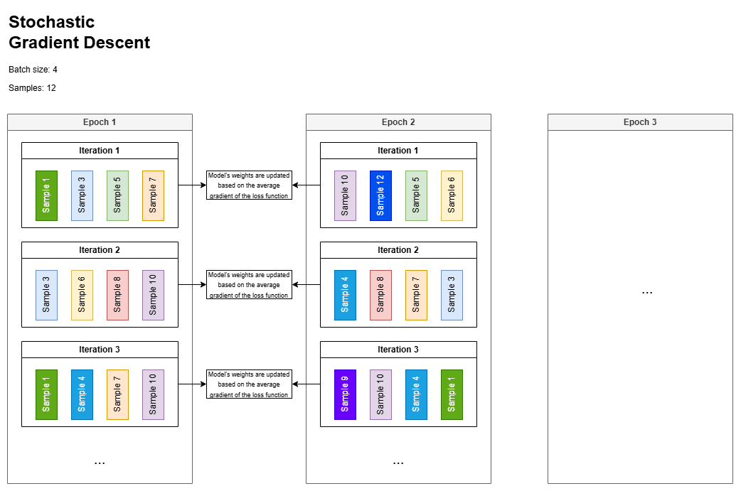
Stochastic Gradient Descent

When using a batch size of 150 during neural network training with backpropagation, each iteration (or step) processes a randomly sampled subset of 150 data points from the dataset. These batches may vary across iterations, especially if shuffling is applied, though some overlap can occur depending on the dataset size and sampling strategy.

In each iteration, the model’s weights are updated based on the average gradient of the loss function computed over the current batch, scaled by the learning rate.

The total number of iterations per epoch is determined by the dataset size and batch size—specifically, it equals ⌈\(N\) / batch_size⌉, where \(N\) is the total number of training examples.

For example, a dataset with 1,000 samples and a batch size of 150 would require 7 iterations per epoch (with the last batch potentially being smaller unless explicitly dropped).

The overall number of iterations in training is then the product of the number of epochs and the iterations per epoch.

Note that one epoch is complete when the model has seen every training sample once (though not necessarily in a single batch).

The role of the optimizer

In the context of Stochastic Gradient Descent (SGD) and its variants (e.g., mini-batch SGD), the optimizer (such as Adam, RMSprop, or SGD with momentum) plays a critical role in determining how the model's weights are updated using the gradients computed during backpropagation. Without an optimizer, vanilla SGD would apply the same fixed learning rate to all weights, which can lead to slow convergence or instability.

Basic SGD (Stochastic Gradient Descent)

• Update rule:

\(w_{t+1} = w_t - \eta \cdot \nabla_w \mathcal{L}(w_t)\)

where \(\eta\) is the learning rate and \(\nabla_w \mathcal{L}\) is the gradient of the loss.

• Limitations:
  • Fixed learning rate for all weights (no adaptation).
  • Sensitive to noisy or sparse gradients.

Advanced Optimizers (e.g., Adam, RMSprop, Momentum)

These introduce adaptive mechanisms to address SGD’s limitations:

1. Momentum-Based (e.g., SGD with Momentum, Nesterov)
   • Idea: Accumulate a moving average of past gradients to dampen oscillations.
   • Effect: Faster convergence through valleys/sharp minima by adding "inertia."

2. Adaptive Learning Rates (e.g., Adam, RMSprop, Adagrad)

   • Idea: Scale the learning rate per parameter based on historical gradient magnitudes.
   • Adam (most popular): Combines momentum (1st moment) and adaptive learning rates (2nd moment) with bias correction.

   \(w_{t+1} = w_t - \eta \cdot \frac{\hat{m}_t}{\sqrt{\hat{v}_t} + \epsilon}\),

   where \(\hat{m}_t\) is momentum and \(\hat{v}_t\) scales the learning rate adaptively.

3. Second-Order Methods (e.g., L-BFGS)
   • Use curvature (Hessian) information for updates (rare in deep learning due to computational cost).

The optimizer decides how to use gradients to update weights, introducing mechanisms like momentum or parameter-specific learning rates to make SGD more efficient and stable. Adam is often the default choice due to its adaptivity, but vanilla SGD (with tuning) can still outperform it in certain scenarios (e.g., training LLMs).

Lottery Ticket Hypothesis with Tensorflow

import tensorflow as tf
from tensorflow.keras.datasets import mnist
from tensorflow.keras.models import Sequential, clone_model
from tensorflow.keras.layers import Dense, Flatten
from tensorflow.keras.utils import to_categorical
import numpy as np
import matplotlib.pyplot as plt
import time

# 1. Load and preprocess data
(x_train, y_train), (x_test, y_test) = mnist.load_data()
x_train, x_test = x_train / 255.0, x_test / 255.0
y_train = to_categorical(y_train)
y_test = to_categorical(y_test)

# 2. Define the original model
def create_model():
    model = Sequential([
        Flatten(input_shape=(28, 28)),
        Dense(400, activation='relu'),
        Dense(300, activation='relu'),
        Dense(10, activation='softmax')
    ])
    return model

# 3. Initialize and train the original model
original_model = create_model()
initial_weights = original_model.get_weights()  # Save the initial random weights
original_model.compile(optimizer='adam', loss='categorical_crossentropy', metrics=['accuracy'])

original_model_learning = original_model.fit(x_train, y_train, epochs=4, batch_size=128, validation_split=0.1)

Epoch 1/4
[1m422/422[0m [32m━━━━━━━━━━━━━━━━━━━━[0m[37m[0m [1m7s[0m 14ms/step - accuracy: 0.8731 - loss: 0.4482 - val_accuracy: 0.9650 - val_loss: 0.1220
Epoch 2/4
[1m422/422[0m [32m━━━━━━━━━━━━━━━━━━━━[0m[37m[0m [1m9s[0m 11ms/step - accuracy: 0.9712 - loss: 0.0939 - val_accuracy: 0.9727 - val_loss: 0.0854
Epoch 3/4
[1m422/422[0m [32m━━━━━━━━━━━━━━━━━━━━[0m[37m[0m [1m6s[0m 14ms/step - accuracy: 0.9828 - loss: 0.0571 - val_accuracy: 0.9785 - val_loss: 0.0738
Epoch 4/4
[1m422/422[0m [32m━━━━━━━━━━━━━━━━━━━━[0m[37m[0m [1m5s[0m 11ms/step - accuracy: 0.9881 - loss: 0.0382 - val_accuracy: 0.9770 - val_loss: 0.0837

# 4. Prune the model (simple magnitude-based pruning)
def prune_weights(model, pruning_percent=0.5):
    weights = model.get_weights()
    new_weights = []
    for w in weights:
        if len(w.shape) > 1:  # only prune dense layer weights
            threshold = np.percentile(np.abs(w), pruning_percent * 100)
            mask = np.abs(w) > threshold
            w = w * mask  # zero out the small weights
        new_weights.append(w)
    return new_weights

pruned_weights = prune_weights(original_model, pruning_percent=0.5)

# 5. Reinitialize model with original random weights and apply the mask (winning ticket)
winning_ticket_model = create_model()
winning_ticket_model.set_weights(initial_weights)
masked_weights = prune_weights(winning_ticket_model, pruning_percent=0.4)
winning_ticket_model.set_weights(masked_weights)

# 6. Retrain the pruned model (winning ticket)
winning_ticket_model.compile(optimizer='adam', loss='categorical_crossentropy', metrics=['accuracy'])
winning_ticket_model_learning = winning_ticket_model.fit(x_train, y_train, epochs=4, batch_size=128, validation_split=0.1)

Epoch 1/4
[1m422/422[0m [32m━━━━━━━━━━━━━━━━━━━━[0m[37m[0m [1m7s[0m 14ms/step - accuracy: 0.8732 - loss: 0.4575 - val_accuracy: 0.9715 - val_loss: 0.0985
Epoch 2/4
[1m422/422[0m [32m━━━━━━━━━━━━━━━━━━━━[0m[37m[0m [1m9s[0m 11ms/step - accuracy: 0.9701 - loss: 0.1006 - val_accuracy: 0.9773 - val_loss: 0.0757
Epoch 3/4
[1m422/422[0m [32m━━━━━━━━━━━━━━━━━━━━[0m[37m[0m [1m6s[0m 14ms/step - accuracy: 0.9824 - loss: 0.0573 - val_accuracy: 0.9795 - val_loss: 0.0659
Epoch 4/4
[1m422/422[0m [32m━━━━━━━━━━━━━━━━━━━━[0m[37m[0m [1m5s[0m 11ms/step - accuracy: 0.9882 - loss: 0.0391 - val_accuracy: 0.9810 - val_loss: 0.0705

# 7. Evaluate both models
print("Original model performance:")
original_model.evaluate(x_test, y_test)

print("Winning ticket model performance:")
winning_ticket_model.evaluate(x_test, y_test)

Original model performance:
[1m313/313[0m [32m━━━━━━━━━━━━━━━━━━━━[0m[37m[0m [1m1s[0m 3ms/step - accuracy: 0.9677 - loss: 0.1016
Winning ticket model performance:
[1m313/313[0m [32m━━━━━━━━━━━━━━━━━━━━[0m[37m[0m [1m1s[0m 3ms/step - accuracy: 0.9738 - loss: 0.0804

[0.07047921419143677, 0.977400004863739]

# Get the weights of the layer (Dense(100, activation='relu'))
print(original_model.layers[1].get_weights()[0].shape)
original_model.layers[1].get_weights()[0]  # Shape: (input_dim, output_dim)

(784, 400)

array([[-0.05667121,  0.02065124, -0.04778236, ...,  0.05302081,
        -0.06146147,  0.00401637],
       [ 0.00472874,  0.00062283, -0.06726848, ..., -0.01869787,
         0.00495344,  0.01626997],
       [-0.06472269,  0.06735108,  0.01358175, ...,  0.00604779,
        -0.04576658,  0.02837193],
       ...,
       [ 0.05708074,  0.05192086,  0.04327519, ..., -0.05372921,
         0.06987718,  0.01477351],
       [ 0.05564093, -0.06744465, -0.01727122, ..., -0.03752626,
         0.01364662,  0.01879197],
       [ 0.04817592,  0.00282612, -0.04398317, ...,  0.04413202,
        -0.01568541, -0.02512715]], dtype=float32)

# Get the weights of the layer
weights = winning_ticket_model.layers[1].get_weights()[0]  # Shape: (input_dim, output_dim)

# Create a boolean mask for weights == 0
zero_mask = (np.abs(weights) == 0)

# Optional: Count the percentage of zeros
sparsity = np.mean(zero_mask) * 100
print(f"Sparsity: {sparsity:.2f}% of weights are exactly zero")

# Visualize the mask (e.g., as a heatmap)
import matplotlib.pyplot as plt
plt.imshow(zero_mask, cmap='gray', interpolation='none')
plt.title("Mask of Zero Weights (White = Zero)")
plt.colorbar()
plt.show()

Sparsity: 4.46% of weights are exactly zero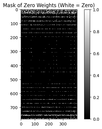

Generative Models Overview

Discriminative vs. Generative Models

• Discriminative models learn to distinguish between different classes or categories. They model the decision boundary between classes and are typically used for classification tasks.
• Generative models, on the other hand, learn the underlying distribution of the data to generate new, similar data points. They describe how data is generated in a probabilistic manner.

Key Characteristics of Generative Models:

• Accept random noise as input and produce new, unique samples.
• Typically unsupervised (do not require labeled data).
• Probabilistic rather than deterministic—randomness enables the generation of diverse outputs.
• Applications include:
  • Data augmentation for imbalanced datasets.
  • Imputation of missing values.
  • Anonymization of sensitive data (producing realistic but non-identifiable samples).

Two Major Types Covered:

• Generative Adversarial Networks (GANs) – Introduced by Ian Goodfellow in 2014.
• Denoising Diffusion Probabilistic Models (DDPMs) – Introduced by Jonathan Ho et al. in 2020.

Generative Adversarial Networks (GANs)

GANs consist of two neural networks in competition:

• Generator (G): Learns to produce realistic data (e.g., images) from random noise.
• Discriminator (D): Learns to distinguish between real data and data generated by the generator.

This setup forms a zero-sum game where:

• The generator tries to fool the discriminator.
• The discriminator tries to correctly identify real vs. fake data.

Training dynamics:

• Initially, the discriminator easily detects fake data.
• Over time, the generator improves, producing more realistic samples.
• Ideally, training reaches a point where the discriminator cannot distinguish real from fake (50% accuracy).

Applications:

• Image generation (e.g., human faces, cartoons).
• Text-to-image translation (e.g., generating images from descriptions).
• Image inpainting (e.g., filling in missing or blurred parts).
• 3D object generation from 2D images.

Denoising Diffusion Probabilistic Models (DDPMs)

Core Concept

• DDPMs generate high-quality images through a two-step process:
  1. Forward diffusion: Gradually adds noise to an image over several steps.
  2. Reverse diffusion: A neural network learns to reverse this process, removing noise step-by-step to reconstruct the image.

Key Features:

• Capable of producing highly detailed and realistic images.
• Do not require labeled data—also an unsupervised learning method.
• Often more stable to train than GANs.

GAN Architecture

The architecture of a GAN consists of two main components:

• Generator (G): Takes random noise as input and generates synthetic (fake) images.
• Discriminator (D): Receives both real images (from the training dataset) and fake images (from the generator), and learns to classify them as real or fake.

The training process is adversarial:

• The generator tries to produce images that are indistinguishable from real ones.
• The discriminator tries to correctly identify which images are real and which are generated.

Training Process

Training Dynamics:

• Initially, the discriminator easily distinguishes real from fake.
• As training progresses, the generator improves, making it harder for the discriminator to tell the difference.
• Ideally, the discriminator's accuracy approaches 50%, meaning it can no longer reliably distinguish real from fake—indicating a well-trained generator.

Loss functions: GANs use two separate loss functions:

• Discriminator Loss: Encourages the discriminator to:
  • Maximize the probability of correctly classifying real images as real.
  • Minimize the probability of misclassifying fake images as real.
• Generator Loss: Encourages the generator to:
  • Maximize the probability that fake images are classified as real by the discriminator.

Both networks are trained using backpropagation.

Common Loss Functions

• Binary Cross-Entropy (BCE): Measures the difference between predicted probabilities and actual labels. It heavily penalizes misclassifications.
• Minimax Loss (original GAN formulation): Can lead to vanishing gradients early in training.
• Wasserstein Loss (WGAN): Improves training stability by replacing the discriminator with a critic that outputs a real-valued score instead of a probability.

Common Challenges in GAN Training

Vanishing Gradients

• Occurs when the discriminator becomes too strong early in training.
• The generator receives little to no gradient information, making it hard to improve.
• Solutions:
  • Use Wasserstein loss instead of minimax.
  • Apply gradient penalty or label smoothing.

Mode Collapse

• The generator produces limited types of outputs (e.g., the same image repeatedly) to fool the discriminator.
• Fails to capture the diversity of the real dataset.
• Solutions:
  • Use Wasserstein loss.
  • Implement Unrolled GANs, where the generator anticipates future discriminator updates.
  • Apply mini-batch discrimination or feature matching.

Failure to Converge

• The generator and discriminator fail to reach equilibrium.
• The discriminator may become too weak or too strong, leading to unstable training.
• Symptoms: Generator quality degrades, discriminator gives random feedback.
• Solutions:
  • Add noise to discriminator inputs.
  • Apply weight regularization to prevent overfitting.
  • Use learning rate scheduling or two-time scale update rules (TTUR).

⚠️ Note: These problems are still active areas of research. No universal solution exists, and training GANs often requires careful tuning and experimentation.

TensorFlow Implementation

Generator model:

generator = tf.keras.Sequential()
generator.add(layers.Dense(64, input_dim=100))
generator.add(layers.ReLU())

generator.add(layers.Dense(128))
generator.add(layers.ReLU())

generator.add(layers.Dense(256))
generator.add(layers.ReLU())

generator.add(layers.Dense(784, activation='tanh'))
generator.add(layers.Reshape((28,28,1)))

The generator is a simple sequential model where each layer is a neural network followed by the ReLU activation function. For more details about activation functions, see My notes about Deep Learning.

The model is designed for the Fashion-MNIST dataset, a collection of grayscale fashion images similar to the classical MNIST. Key characteristics:

• Input: Random noise (100 dimensions)
• Architecture: Progressive expansion from 64 → 128 → 256 neurons
• Output: 784 neurons (28×28 pixels) with tanh activation to fit the range [-1, 1]
• Reshape: Final layer outputs 28×28 grayscale images

The generator contains approximately 250,000 trainable parameters.

Generating images from noise:

# Generate latent noise vector
noise = tf.random.normal([1, 100])
generated_image = generator(noise, training=False)

# Display the generated image
plt.imshow(generated_image[0,:,:,0], cmap='gray')

The noise vector follows a Gaussian distribution with 100 dimensions. Setting training=False shows generator output without further training.

Discriminator model:

discriminator = tf.keras.Sequential()
discriminator.add(layers.Input(shape=(28,28,1)))
discriminator.add(layers.Flatten())

discriminator.add(layers.Dense(256))
discriminator.add(layers.LeakyReLU(0.2))
discriminator.add(layers.Dropout(0.5))

discriminator.add(layers.Dense(128))
discriminator.add(layers.LeakyReLU(0.2))
discriminator.add(layers.Dropout(0.3))

discriminator.add(layers.Dense(64))
discriminator.add(layers.LeakyReLU(0.2))
discriminator.add(layers.Dropout(0.2))

discriminator.add(layers.Dense(1, activation='sigmoid'))

The discriminator is a binary classification model that determines whether input images are real or fake:

• Input: 28×28 grayscale images (flattened)
• Activation: LeakyReLU (α=0.2) provides better GAN performance by allowing slight gradients for negative inputs
• Regularization: Dropout layers prevent overfitting
• Output: Sigmoid activation ensures probability scores between 0-1

Testing the Discriminator:

output = discriminator(generated_image)

An untrained discriminator typically outputs scores around 0.5 (50%), indicating it cannot distinguish real from fake images.

Loss Functions

Binary Cross-Entropy Setup:

bce = tf.keras.losses.BinaryCrossentropy()

Binary cross-entropy heavily penalizes misclassifications and is suitable for both discriminator training and generator adversarial training.

Discriminator Loss:

def discriminator_loss(real_output, fake_output):
    real_loss = bce(tf.ones_like(real_output), real_output)
    fake_loss = bce(tf.zeros_like(fake_output), fake_output)
    total_loss = real_loss + fake_loss
    return total_loss

The discriminator loss encourages:

• Real data classification as 1 (true)
• Fake data classification as 0 (false)

Generator Loss:

def generator_loss(fake_output):
    gen_loss = bce(tf.ones_like(fake_output), fake_output)
    return gen_loss

The generator loss encourages the discriminator to classify fake images as real (1), effectively "fooling" the discriminator.

Optimizers and Checkpointing:

# Setup optimizers
generator_optimizer = Adam(learning_rate=0.001)
discriminator_optimizer = Adam(learning_rate=0.001)

# Create checkpoint for model saving
checkpoint = tf.train.Checkpoint(
    generator_optimizer=generator_optimizer,
    discriminator_optimizer=discriminator_optimizer,
    generator=generator,
    discriminator=discriminator
)

The Adam optimizer uses an exponentially weighted average of gradients and has proven effective in real-world applications. The checkpoint system ensures model persistence during training interruptions.

Training Process

Setup Parameters:

# Training configuration
EPOCHS = 50
noise_dim = 100
num_examples_to_generate = 16

# Generate consistent seed for visualization
seed = tf.random.normal([num_examples_to_generate, noise_dim])

The training process requires defining key parameters:

• EPOCHS: Number of complete passes through the dataset
• noise_dim: Dimensionality of input noise vector (100 dimensions)
• num_examples_to_generate: Number of sample images to generate for progress visualization

Training Step Function:

@tf.function
def train_step(images):
  noise = tf.random.normal([BATCH_SIZE, noise_dim])

  with tf.GradientTape() as gen_tape, tf.GradientTape() as disc_tape:
    # Generate fake images
    generated_images = generator(noise, training=True)

    # Get discriminator outputs
    real_output = discriminator(images, training=True)
    fake_output = discriminator(generated_images, training=True)

    # Calculate losses
    disc_loss = discriminator_loss(real_output, fake_output)
    gen_loss = generator_loss(fake_output)

  # Compute gradients
  gradients_of_generator = gen_tape.gradient(gen_loss, generator.trainable_variables)
  gradients_of_discriminator = disc_tape.gradient(disc_loss, discriminator.trainable_variables)

  # Apply gradients
  generator_optimizer.apply_gradients(zip(gradients_of_generator, generator.trainable_variables))
  discriminator_optimizer.apply_gradients(zip(gradients_of_discriminator, discriminator.trainable_variables))

  return gen_loss, disc_loss, tf.reduce_mean(real_output), tf.reduce_mean(fake_output)

Key aspects of the training step:

• @tf.function decorator: Converts Python code into a TensorFlow computation graph for improved performance
• Dual GradientTape: Simultaneously tracks gradients for both generator and discriminator
• Separate optimization: Each network is updated independently using its respective optimizer

Progress Visualization:

def generate_and_plot_images(model, epoch, test_input):
  predictions = model(test_input, training=False)

  fig = plt.figure(figsize=(4, 4))
  for i in range(predictions.shape[0]):
    plt.subplot(4, 4, i+1)
    plt.imshow(predictions[i, :, :, 0] * 127.5 + 127.5, cmap='gray')
    plt.axis('off')

  plt.savefig('image_at_epoch_{:04d}.png'.format(epoch))
  plt.show()

This function generates a 4×4 grid of sample images to visualize generator progress throughout training.

Main Training Loop:

def train(dataset, epochs):
  for epoch in range(epochs):
    start = time.time()

    # Track losses for the epoch
    gen_loss_epoch = []
    disc_loss_epoch = []
    real_accuracy_epoch = []
    fake_accuracy_epoch = []

    for image_batch in dataset:
      gen_loss, disc_loss, real_acc, fake_acc = train_step(image_batch)

      # Collect metrics
      gen_loss_epoch.append(gen_loss)
      disc_loss_epoch.append(disc_loss)
      real_accuracy_epoch.append(real_acc)
      fake_accuracy_epoch.append(fake_acc)

    # Calculate average metrics
    avg_gen_loss = tf.reduce_mean(gen_loss_epoch)
    avg_disc_loss = tf.reduce_mean(disc_loss_epoch)
    avg_real_acc = tf.reduce_mean(real_accuracy_epoch)
    avg_fake_acc = tf.reduce_mean(fake_accuracy_epoch)

    # Generate sample images
    generate_and_save_images(generator, epoch + 1, seed)

    # Save checkpoint every 15 epochs
    if (epoch + 1) % 15 == 0:
      checkpoint.save(file_prefix=checkpoint_prefix)

    print(f'Epoch {epoch+1}/{epochs}:')
    print(f'  Generator Loss: {avg_gen_loss:.4f}')
    print(f'  Discriminator Loss: {avg_disc_loss:.4f}')
    print(f'  Real Accuracy: {avg_real_acc:.4f}')
    print(f'  Fake Accuracy: {avg_fake_acc:.4f}')
    print(f'  Time: {time.time()-start:.2f} sec')

Training Execution:

# Execute training
train(train_dataset, EPOCHS)

Training Results and Analysis:

During training, several key observations emerge:

Progressive Image Quality:

• Early epochs produce blurry, noise-like images
• Middle epochs show recognizable shapes and patterns
• Later epochs generate increasingly realistic fashion items

Loss Dynamics:

• Generator loss typically decreases as it learns to fool the discriminator
• Discriminator loss may fluctuate as it adapts to improving generator outputs
• Ideal training shows both losses stabilizing rather than one completely dominating

Accuracy Metrics:

• Real accuracy: Discriminator's ability to correctly identify real images
• Fake accuracy: Discriminator's ability to correctly identify fake images
• As training progresses, discriminator performance may slightly degrade (closer to 50%) indicating the generator is successfully learning

Performance Notes

While fully connected layers can generate recognizable images, Convolutional Neural Networks (CNNs) typically produce superior results for image generation tasks due to their ability to:

• Preserve spatial relationships
• Learn hierarchical features
• Handle translation invariance more effectively

The training process demonstrates the adversarial dynamics where the generator progressively improves while the discriminator's task becomes increasingly challenging.

Building a GAN using Deep Convolutional Networks

Convolutional Neural Networks perform better for images. They capture spatial features of images and are sparse neural networks that work in the original dimensions.

Standard Convolutional Layers

Standard convolutional layers are made up of two components:

Convolutional Layer

The convolutional layer involves sliding a kernel over the input image to extract features:

• Kernel weights are learned during the training process
• Used to extract features from the underlying image
• Generate feature map representations of the input image

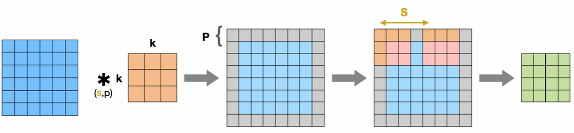
Process:

• Input: Image with height, width, and number of channels
• Kernel: A k×k filter that slides across the image
• Zero padding: Additional zero values around the images to control the size of the output feature map
• Stride: The step size (horizontal and vertical) with which the kernel moves over the image
• Feature extraction: Kernel weights are multiplied by underlying image values to generate feature maps

Output Size Formula: \($o=\frac{i+2p-k}{s} + 1\)$

Where:

• i: Size of the input image
• p: Size of the zero padding
• k: Size of kernel
• s: Stride
• o: Size of the output

Pooling Layer

Reduces the spatial dimensions of the input through aggregating operations:

• Purpose: Reduces the number of parameters the network has to process
• Common types: Average pooling, max pooling
• Effect: Downsamples feature maps while retaining important information

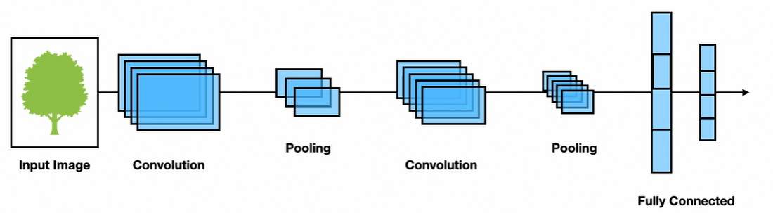
The output from these layers typically feeds into fully connected dense layers for final tasks like classification or segmentation.

Advanced Convolutional Operations

Deconvolutional Layers

• Purpose: Reverse the operation of standard convolutional layers
• Function: Takes feature maps as input and produces representations closer to the original input dimensions

Transposed Convolutional Layers

Perform upsampling of input data to generate output feature maps with spatial dimensions greater than the input:

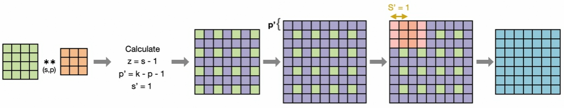
Process:

• Start with input map and kernel with modified stride and padding parameters
• z: Number of zeros inserted between rows and columns of the input (shown as purple cells)
• p': Zero padding added around the image
• s': Kernel stride (always 1 for transposed convolutions)
• Output: Upsampled image with increased spatial dimensions

Output Size Formula: \($o=(i-1) \times s + k - 2p\)$

Deep Convolutional GANs (DCGANs)

DCGANs are similar to regular GANs but use convolutional networks with specific architectural constraints. These constraints help the adversarial networks learn hierarchical representations, resulting in better generated images.

Original Research: Introduced by Alec Radford et al. in 2016.

Replace Pooling with Strided Convolutions:

• Pooling layers were found to hurt model convergence
• Use strided convolutional layers for downsampling in discriminator
• Use transposed convolutions for upsampling in generator

Batch Normalization:

• Applied to generator and discriminator layers
• Benefits:
  • Recenters layer outputs to have zero mean and unit variance
  • Mitigates poor initialization issues
  • Helps with vanishing gradients in deeper networks
  • Prevents mode collapse
• Exceptions: Not applied to generator output layer and discriminator input layer

Remove Fully-Connected Hidden Layers:

• Eliminates fully-connected layers in deeper architectures
• Generator uses single-dimensional noise input reshaped to 4D tensor
• Creates the foundation for the convolutional stack

Activation Functions:

• Generator: ReLU activation for all layers except the output layer, which uses tanh to generate pixel values in range [-1, 1]
• Discriminator: LeakyReLU activation throughout the network

DCGAN Architecture

Generator Architecture: The generator transforms single-dimensional noise input through progressive upsampling:

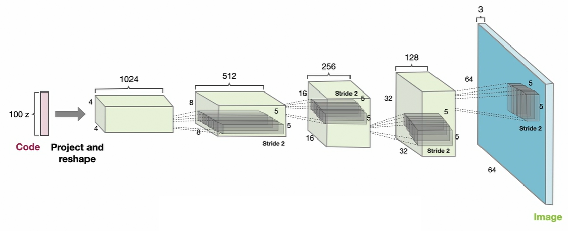
• Input: Random noise vector
• Process: Projected and reshaped through strided convolutional layers
• Output: Upsampled image with realistic features

Discriminator Architecture: The discriminator processes input images through progressive downsampling:

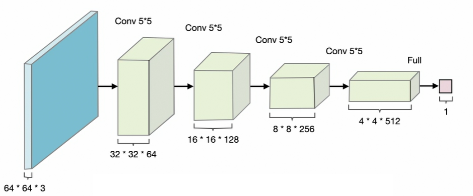
• Input: Real or generated images
• Process: Downsampling through convolutional layers
• Output: Single probability value indicating whether input is real or fake

This architecture enables DCGANs to generate higher quality images compared to fully-connected GANs while maintaining training stability through the carefully designed constraints.

Training of the Deep Convolutional GANs

It's the same code of the previous example with the fully connected GANs, but with different models of the generator and the discriminator.

• Load the Fashion MNIST dataset:

from tensorflow.keras.datasets import fashion_mnist
# 6000 images each 28x28 grayscale
(train_images, ), (, _) = fashion_mnist.load_data()
# Reshape so that each image has the dimension 28x28x1
train_images = train_images.reshape(train_images.shape[0], 28, 28, 1).astype('float32')
# Normalize to [-1,1]
train_images = (train_images - 127.5) / 127.5

• Construct the Generator model:

from tensorflow.keras import layers, models

def generator_model():
  model = models.Sequential()
  # This dimension is because the input is a batch of noise where each vector as 100 neurons 
  model.add(layers.Dense(7 * 7 * 256, use_bias=False, input_shape=(100,)))
  # Resample data to have mean of zero and variance of one
  model.add(layers.BatchNormalization())

  model.add(layers.ReLU())

  # Reshape in four dimensions, batch is the first and the remining three are 7,7, and 256
  model.add(layers.Reshape((7, 7, 256)))

  # Transpose convolutionals layer to upsample
  model.add(layers.Conv2DTranspose(128, (5, 5), strides=(1, 1), padding='same', use_bias=False))
  model.add(layers.BatchNormalization())
  model.add(layers.ReLU())
  model.add(layers.Conv2DTranspose(64, (5, 5), strides=(2, 2), padding='same', use_bias=False))
  model.add(layers.BatchNormalization())
  model.add(layers.ReLU())

  # Produces an uspsample image of the same size from real dataset - tanh activation ensures the range -1,1
  model.add(layers.Conv2DTranspose(1, (5, 5), strides=(2, 2), padding='same', use_bias=False, activation='tanh'))

  return model

• Constructing the Discriminator Model:

  def discriminator_model():
  model = models.Sequential()
  # Input shape is 28x28x1 again
  model.add(layers.Conv2D(64, (5, 5), strides=(2, 2), padding='same', input_shape=[28, 28, 1]))
  
  model.add(layers.BatchNormalization())
  model.add(layers.LeakyReLU(0.2))
  model.add(layers.Dropout(0.3))
  
  # Same architecture
  model.add(layers.Conv2D(128, (5, 5), strides=(2, 2), padding='same'))
  model.add(layers.BatchNormalization())
  model.add(layers.LeakyReLU(0.2))
  model.add(layers.Dropout(0.3))
  
  # Flattens the image to output a probability score (image is real or less?)
  model.add(layers.Flatten())
  model.add(layers.Dense(1, activation='sigmoid'))
  return model

Feel free to tweak the batch size and other parameters to see how the training process changes.

Setting up the Loss Functions and Optimizers.

• Loss Functions

  • Binary Cross-Entropy Loss: Used as the base loss function with from_logits=True for numerical stability
  • Discriminator Loss: Combines losses from real and fake samples
  • Real loss: Measures how well the discriminator identifies real images (target: 1)
  • Fake loss: Measures how well the discriminator identifies fake images (target: 0)
  • Total loss: Sum of real and fake losses
  • Generator Loss: Measures how well the generator fools the discriminator by trying to make fake images appear real (target: 1)

• Optimizers

  • Adam Optimizers: Both generator and discriminator use Adam optimization with:
  • Learning rate: 0.0002 (commonly used for GAN training)
  • Beta_1: 0.5 (lower momentum for better GAN stability)

cross_entropy = tf.keras.losses.BinaryCrossentropy(from_logits=True)

def discriminator_loss(real_output, fake_output):
  real_loss = cross_entropy(tf.ones_like(real_output), real_output)
  fake_loss = cross_entropy(tf.zeros_like(fake_output), fake_output)
  total_loss = real_loss + fake_loss
  return total_loss

def generator_loss(fake_output):
  return cross_entropy(tf.ones_like(fake_output), fake_output)

generator_optimizer = tf.keras.optimizers.Adam(learning_rate=0.0002, beta_1=0.5)
discriminator_optimizer = tf.keras.optimizers.Adam(learning_rate=0.0002, beta_1=0.5)

Training Step Function:

@tf.function
def train_step(images):
noise = tf.random.normal([BATCH_SIZE, noise_dim])

with tf.GradientTape() as gen_tape, tf.GradientTape() as disc_tape:
  generated_images = generator(noise, training=True)

  real_output = discriminator(images, training=True)
  fake_output = discriminator(generated_images, training=True)

  gen_loss = generator_loss(fake_output)
  disc_loss = discriminator_loss(real_output, fake_output)

  gradients_of_generator = gen_tape.gradient(gen_loss, generator.trainable_variables)
  gradients_of_discriminator = disc_tape.gradient(disc_loss, discriminator.trainable_variables)

  generator_optimizer.apply_gradients(zip(gradients_of_generator, generator.trainable_variables))
  discriminator_optimizer.apply_gradients(zip(gradients_of_discriminator, discriminator.trainable_variables))

Training Loop:

def train(dataset, epochs):
  for epoch in range(epochs):
    for image_batch in dataset:
      train_step(image_batch)

      # Produce images for the GIF as you go
      display.clear_output(wait=True)
      generate_and_save_images(generator, epoch + 1, seed)

      # Save the model every 15 epochs
      if (epoch + 1) % 15 == 0:
          checkpoint.save(file_prefix = checkpoint_prefix)

      Generate after the final epoch
      display.clear_output(wait=True)
      generate_and_save_images(generator, epochs, seed)

We can see that it performs better, better quality and faster.

The generator loss chart falls dramatically after just a few epochs of training, while discriminator loss raises. The accuracies scores converge towards 50%.

Training a Deep Convolutional GAN on Multichannel Images

This section highlights only the code differences from the previous chapter, focusing on handling multichannel (color) images.

Loading Multichannel Image Data

When using Google Colab, you can store your data in Google Drive and mount it for access:

from google.colab import drive
drive.mount('/content/drive')

Unzip your training data (for example, a ZIP file of images):

!unzip /content/drive/MyDrive/anime_images_data.zip -d /content

Load the dataset using TensorFlow's image dataset utility:

dataset = tf.keras.preprocessing.image_dataset_from_directory(
  '/content/images',
  labels=None,
  image_size=(64, 64),
  batch_size=128
)

For more complex datasets than Fashion-MNIST, images are typically 64×64 pixels and have 3 color channels (RGB).

Scale image pixel values to the range [-1, 1] (as expected by the GAN):

def scale(image):
  image = tf.cast(image, tf.float32)
  image = (image - 127.5) / 127.5
  return image

Apply this scaling to your dataset:

dataset = dataset.map(scale)

Visualize a batch of training images:

for images in dataset.take(1):
  plt.figure(figsize=(10, 10))
  for i in range(25):
    plt.subplot(5, 5, i + 1)
    plt.imshow((images[i] + 1) / 2)  # Rescale to [0, 1] for display
    plt.axis('off')
  plt.show()

Deep Convolutional GANs for Multichannel (Color) Images

When working with color images (e.g., 64×64 RGB), the DCGAN architecture is adapted to handle the increased complexity and number of channels.

The generator transforms a noise vector into a 64×64×3 color image using a series of upsampling layers:

from tensorflow.keras import layers, models

generator = models.Sequential([
  layers.Dense(4 * 4 * 256, use_bias=False, input_shape=(100,)),
  layers.BatchNormalization(),
  layers.ReLU(),
  layers.Reshape((4, 4, 256)),
  layers.Conv2DTranspose(128, (5, 5), strides=(2, 2), padding='same', use_bias=False),
  layers.BatchNormalization(),
  layers.ReLU(),
  layers.Conv2DTranspose(64, (5, 5), strides=(2, 2), padding='same', use_bias=False),
  layers.BatchNormalization(),
  layers.ReLU(),
  layers.Conv2DTranspose(3, (5, 5), strides=(2, 2), padding='same', use_bias=False, activation='tanh')
])

generator.summary()

• Input: 100-dimensional noise vector
• Dense layer: Projects noise to 4×4×256 tensor
• Batch normalization and ReLU: Applied after each upsampling layer
• Conv2DTranspose layers: Progressively upsample to 8×8, 16×16, and finally 64×64 with 3 channels (RGB)
• Output activation: tanh for pixel values in [-1, 1]

The discriminator classifies 64×64×3 images as real or fake using downsampling convolutional layers:

discriminator = models.Sequential([
  layers.Conv2D(64, (5, 5), strides=(2, 2), padding='same', input_shape=[64, 64, 3]),
  layers.LeakyReLU(alpha=0.2),
  layers.Dropout(0.3),
  layers.Conv2D(128, (5, 5), strides=(2, 2), padding='same'),
  layers.LeakyReLU(alpha=0.2),
  layers.Dropout(0.3),
  layers.Conv2D(256, (5, 5), strides=(2, 2), padding='same'),
  layers.LeakyReLU(alpha=0.2),
  layers.Dropout(0.3),
  layers.Flatten(),
  layers.Dense(1, activation='sigmoid')
])

discriminator.summary()

• Input: 64×64×3 color image
• Conv2D layers: Downsample spatial dimensions and increase feature depth
• LeakyReLU and Dropout: Improve training stability and prevent overfitting
• Flatten and Dense: Output a single probability (real/fake)

Note: All convolutional and transposed convolutional layers use a kernel initializer with mean 0 and standard deviation 0.02, as recommended for DCGANs.

This architecture enables effective training of GANs on color image datasets, such as anime faces or CIFAR-10.

Training Diffusion Models

See Diffusion models in details.

See "awjuliani/pytorch-diffusion" on GitHub as a sample implementation.

• Data.py: Contains the DiffSet class, used to represent and hold the training dataset. It inherits from py.dataset and supports datasets like MNIST, FashionMNIST, and CIFAR10.
• Modules.py: Sets up the neural network layers for the diffusion model.
• Self Attention Layer: Helps neural networks memorize long sequences of input data.
• Double Convolution Layer: Used in the diffusion de-noising process, borrowed from semantic segmentation models.
• Downsampling and Upsampling Layers: Perform downsampling and upsampling of the input image.
• Positional Encoding: Describes the location or position of an entity in a sequence.
• Model.py: Contains the diffusion model class, which inherits from lightning module.
• Init Function: Initializes layers like double convolution, downsampling, upsampling, self attention, and positional encoding.
• Forward Function: Implements the forward diffusion process using self attention layers and positional encodings.
• De-noise Sample Function: Performs the reverse diffusion process, generating a sample from pure noise.

Training Setup:

• Dataset: The MNIST handwritten digit dataset is used.
• Training Parameters: Training runs for 10 epochs with a batch size of 128.
• Model Checkpointing: The model is checkpointed during training to resume from the last checkpoint if needed.
• Data Loaders: Separate loaders for training and validation datasets are set up.
• Training: The model is trained using the PyTorch Lightning trainer class for a maximum of 10 epochs using a GPU.

Generating Images:

• Noise Generation: A batch of pure noise is generated using torch.randn.
• Denoising: The noise is fed into the diffusion model to generate samples.
• Post-Processing: The generated samples undergo post-processing to view the denoised images.
• Results: The model generates images resembling handwritten digits, though the quality varies with the number of training epochs