
- Tensors
- Element-wise multiplication
- MLP
- Transfer functions
- Weight initialization
- Gradient descend
- Backpropagation
- Feed-forward networks
- Convolutional networks
- Recurrent neural networks (RRT)
- Generative Adversarial Networks
- Autoencoders
- Parallel training techniques
- Attention Mechanisms and Bidirectional RNNs
- Diffusion Models
Tensors
Tensors are generalizations of vectors and matrices to higher dimensions. It's a mathematical object that can be represented as a multi-dimensional array of numbers and transforms:
- scalar: zero-dimensional tensor (rank 0),
- vector: one-dimensional tensor (rank 1),
- matrix: two-dimensional tensor (rank 2),
- high-order tensors: \(n\)-dimensional arrays (\(n\)-rank).
The rank of a tensor refers to the number of indices (dimensions) required to uniquely identify each element of the tensor. E.g., rank-3 tensors \(T_{ijk}\).
Notation:
\(T_{i_{1},i_{2}..i_{n}}\)
Tensor contraction: Reducing the rank of a tensor by summing over one or more pairs of indices (e.g., summing \(T_{ij}\) over \(j\)).
Example of Tensor Contraction
Example: Contraction of a \(2\)-rank Tensor (Matrix)
Consider a \(2\)-rank tensor, represented as a matrix \(A\) with components \(A_{ij}\). The contraction involves summing over one pair of indices, such as \(i=j\).
\( A = \begin{bmatrix} a_{11} & a_{12} \\ a_{21} & a_{22} \end{bmatrix} \)
The contraction over \(i\) and \(j\) (i.e., \(\sum_i A_{ii}\)) results in the trace of the matrix:
\( \text{Tr}(A) = A_{11} + A_{22} \)
General Example: Higher-Rank Tensor
For a 3D tensor \(T_{ijk}\), we can contract over any pair of indices. For example, contracting over \(i\) and \(j\):
\( \sum_{i=j} T_{iik} \)
This reduces \(T_{ijk}\), which has rank \(3\), to a tensor \(T_k\), which has rank \(1\) (a vector).
Element-wise multiplication
Given \(A=[[1,2],[3,4]]\) and \(B=[[5,6],[7,8]]\)
\(C=multiply(A,B)=[[1 \cdot 5,2 \cdot 6],[3 \cdot 7,4 \cdot 8]]=[[5,12],[21,32]]\)
In Python:
numpy.multiply(A,B)
MLP
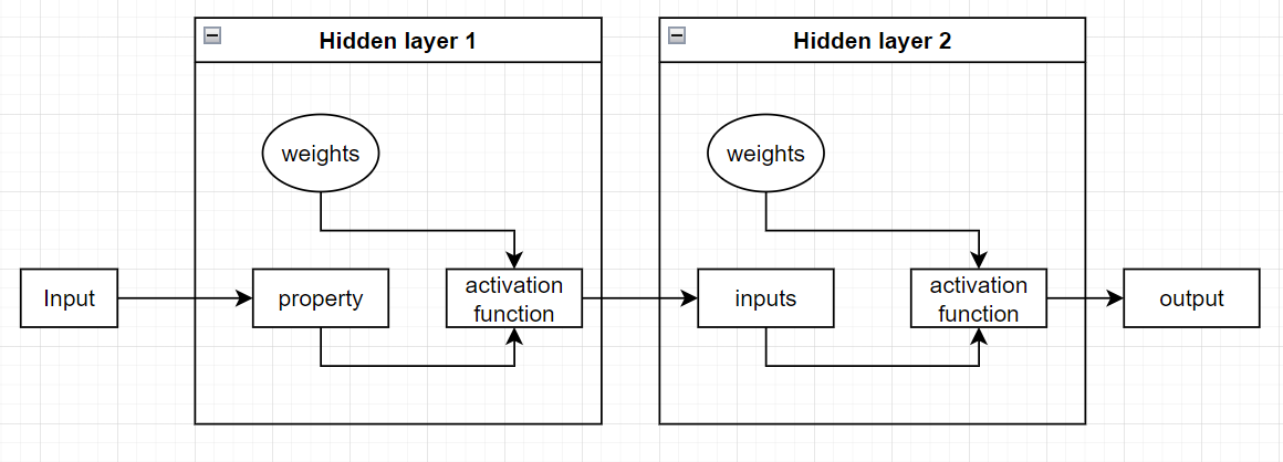
A perceptron is a single-layer neural network. It is the simpliest type of artificial neural network and is a foundational building block in machine learning.
Mathematical Representation of the perceptron:
\(y=f(\sum_{i=1}^n w_i x_i + b)\)
- \(f\): activation function;
- \(w\): weight;
- \(x\): property;
- \(b\): bias.
A typical activation function could be \(f(x)=\{x>0:1, x<0:0\}\)
The perceptron doesn't have the capacity for complex patterns or nonlinear decision boundaries. A MLP with sufficient hidden neurons an approximate any continuous function.
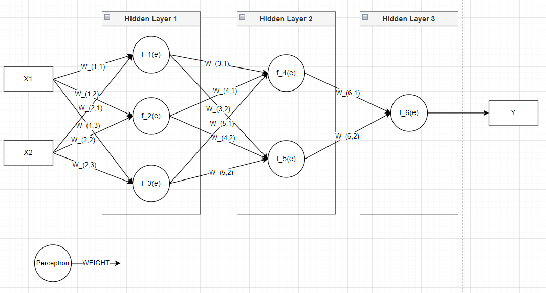
Multi-layer perceptron
A multi-layer perceptron (MLP) is an extension of the perceptron that:
- addresses its limitations by introducing one or more hidden layer,
- can solve complex and non-linear problems.
Hidden layers are an architecture element of MLP consisting in one or more intermediate layers that process the inputs.
The networks that have multiple hidden layers are named deep neural networks.
Mathematical representation for a single hidden layer:
\(z_j=f(\sum_{i=1}^{n}w_{ji}x_i+b_j)\)
\(y_k=g(\sum_{j=1}^{m}v_{kj}z_j+c_k)\)
- \(z_j\): output of the j-th hidden neuron;
- \(y_k\): output of the k-th hidden neuron;
- \(w_{ji}\): weights from input to hidden layer;
- \(v_{kj}\): weights from hidden layer to output;
- \(f,g\): activation functions.
Two hidden layers example: \(z=f(input)\)
\(t=g(z)\)
\(output=h(t)\)
Applications:
- image recognition
- natural language processing
- time series forecasting
- robotics and control systems.
Transfer functions
- The activation function is the feature of the perceptron that applies a threshold or step function to decide the output (0 or 1).
- The transfer function introduce non-linearity to the neural network enabling it to model complex patterns in data.
- A neural network would behave like a simple linear model without non-linearity, regardless of the number of layers.
| Transfer function | Formula | Output range | Usage | Limitations |
|---|---|---|---|---|
| Linear | \(f(x)=x\) | Output layers for regression tasks | Cannot model non-linear relationships | |
| Sigmoid | \(f(x)=\frac{1}{(1+e^{-x})}\) | 0,1 | Probabilities in binary classification tasks | - Not zero-centered (slows down convergence); - Vanishing gradient: outputs are in the range 0,1 and derivatives are very small fro inputs far from 0 |
| Tanh | \(f(x)=\frac{e^x-e^{-x}}{e^x+e^{-x}}\) | -1,1 | Zero-centered (spped up convergence) | Vanishing gradient: outputs are in the range -1,1 and derivatives are very small for large positive or negative inputs. Used occasionally but often replaced by ReLU |
| ReLU (Rectified Linear Unit) | \(f(x)=max(0,x)\) | Computationally efficient. Solve vanishing gradient for positive inputs. Default choice for most hidden layers (included variants). | Can cause dead neurons if weights are initialized poorly leading to zero gradients | |
| Leaky ReLU | \(f(x)=\{x>0: f(x)=x, x \le 0: f(x)=\alpha x\}\) with \(\alpha>0\) | Addresses the dead neuron problem by allowing small gradients for negative inputs | ||
| Softmax | \(f(x_i)=\frac{e^{x_i}}{\sum_{j=1}^n e^{x_j}}\) where \(i\) is the class | Used in output layers for multi-class classfication | ||
| SELU (Scaled Exponential Linear Unit) | Designed for self-normalizing networks. Maintain mean and variance during training |
Weight initialization
Weight initialization is important in deep learning to:
- avoid vanishing or exploding gradients,
- faster convergence: reduce the number of iterations required to reach convergence,
- symmetry breaking: prevents neurons in the same layer from learning identical features by starting with slightly different weights.
Weight initializations:
- Zero initialization: cause that alle neurons learn the same features leading to symmetry problems,
- Random Initialization: lead to vanishing or exploding gradients in deep networks,
- He initialization: ensure that the gradients remain stable in deep networks with ReLU activations.
- The weights in the He initialization are drawn from a distribution with variance \(\frac{2}{n_{in}}\) where \(n_{in}\) is the number of inputs to a neuron.
- It's practice for ReLU activation function or its variants (Leaky ReLU, PReLU).
- Xavier initialization: maintain variance across layers for smooth gradient flow in deep networks with sigmoid or tanh activations.
- The weights in the Xavier initialization are drawn from a distribution with variance \(\frac{1}{n_{in}}\) where \(n_{in}\) is the number of inputs to a neuron.
- It's practice for sigmoid or tanh activation functions.
- Lecun initialization: it's practice for SELU activation functions.
Choosing the right weight initialization and transfer function is critical for effective neural network training.
Gradient descend
Optimization algorithm used to minimize a loss function (i.e., the difference between predicted and actual values).
- Iteratively update the model's parameters (weights and biases) in the opposite direction of the gradient of the loss function with respect to the parameters.
Steps:
- Initialization: start with random values for the parameters (weights and biases) (or, I suppose, based on weight initialization).
- Compute the gradient: calculate the gradient of the loss function with respect to each parameter.
- Update parameters: adjust the parameters in the direction opposite to the gradient to reduce the loss:
\(\theta \leftarrow \theta - \lambda \cdot \nabla J(\theta)\)
- \(\theta\): parameters (weights, biases),
- \(\lambda\): learning rate (size of the steps),
- \(\nabla J(\theta)\): gradient of the loss function with respect to \(\theta\).
Then repeat the process until convergence (loss function reaches a minimum).
Variants of Gradient descend:
- Batch Gradient Descent: Uses the entire dataset to compute the gradient.
- Stochastic Gradient Descent (SGD): Updates parameters using one data point at a time.
- Mini-batch Gradient Descent: Combines the benefits of batch and stochastic by using small batches of data.
Backpropagation
The learning algorithm used by MLP to adjust weights using the error gradient.
- During a back pass is used the chain rule to calculate the gradients layer by layer.
Steps:
- Forward pass: input data flows through the network to compute predictions.
- Calculate activations for each layer.
- Compute the loss using the predictions and actual values.
- Backward Pass: Compute the gradient of the loss function with respect to each weight and bias.
- Start at the output layer and calculate the gradient of the loss with respect to the output.
- Propagate the error backward through the network using the chain rule to compute gradients for earlier layers.
- Weight Updates: Use the gradients calculated in the backward pass with Gradient Descent to update the weights.
Key Concepts:
- Chain Rule: Enables the calculation of gradients layer by layer.
- Partial Derivatives: Measure the sensitivity of the loss to changes in each parameter.
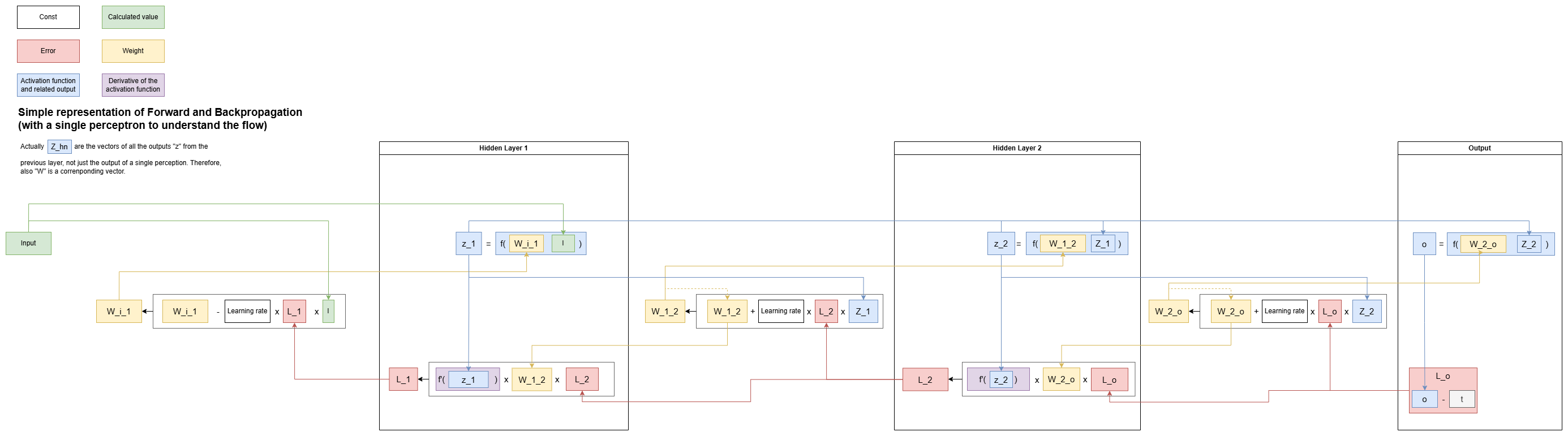
Representation of backpropagation with a single perceptron to help understanding
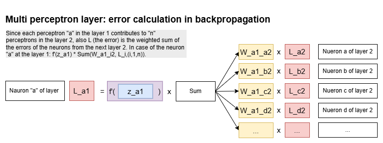
Representation of error calculation for a single perceptron simplified
Example for a neural network
- Forward pass:
- Prediction = \(y=f(Wx+b)\).
- Compute the loss: \(L(y-\hat{y})\) (where \(\hat{y}\) is the actual value).
- Backward pass using Backpropagation: compute gradients (partial derivative of the loss function with respect to the parameters) \(\frac{\partial L}{\partial W}\), \(\frac{\partial L}{\partial W}\).
- Gradient Descent: update \(W\) and \(b\):
-
\(W \leftarrow W - \lambda \frac{\partial L}{\partial W}\)
\(b \leftarrow b - \lambda \frac{\partial L}{\partial b}\)
This process trains the network by iteratively reducing the loss.
Vanishing gradient
The vanishing gradient problem happens more often in networks with many layers.
ReLU help prevent the vanishing gradient problem for positive inputs. ReLU neurons can stop learning if their inputs are always negative.
Example of a vanishing gradient in a 3-layer neural network with the sigmoid activation function:
\(Input \rightarrow Hidden layer 1 \rightarrow Hidden layer 2 \rightarrow Output\)
Derivative of the sigmoid (calcuated in the Machine Learning sheet): \(\frac{d\phi(z)}{dz}=\phi(z)(1-\phi(z))\)
This derivative (gradient) will assume the values \(0\) - \(0,25\). Example: \(0.5 \cdot (1-0.5)=0.5 \cdot 0.5=0.25\)
Assuming that the network is performing backpropagation to update the weights, the gradient of the loss \(L\) with respect to a weight \(W\) in a specific layer would be the product of gradients from all previous layers, due to the chain rule: \(\frac{dL}{W}=\)=gradient of layer 2 \(\cdot\) gradient of alyer 3 \(\cdot\) ... \(\cdot\) gradent of layer n.
Taking the example of the gradient above, the gradients (derivatives of the sigmoid) at each layer would be:
- layer3: \(0.25\)
- layer2: \(0.25\)
- layer1: \(0.25\)
Using the chain rule, the gradient calculated at Layer 1:
\(0.25 \cdot 0.25 \cdot 0.25 = 0.015\)
In deeper networks (e.g. 10+ layers) multiplying many small gradients (values \(<1\)) would lead to gradient approaching \(0\).
When gradient approaches \(0\), the weights in the earlier layers stop updating effectively during backpropagation. The network cannot learn effectively because weights updates (proportional to the gradient) become negligible.
The ReLU activation function would solve for positive values because if \(x>0\): \(\frac{d max(0,x)}{dx}=\frac{dx}{dx}=1\)
Feed-forward networks
Feed-forward networks are neural network consitent in layers of neurons where information flows in one direction (from the input layer, through hidden layers, to the output layer) and there are no cycles or loops. The main advantage is that they are easy to implement and understand.
- A single neuron with a linear or continuous activation function correspond to a regression.
- Each neuron in the input layer corresponds to one feature in the dataset.
- One or more neurons with a softmax or sigmoid activation in a feed-forward network correspond to the classification task.
Limitations:
- It doesn't retain memory of previous inputs (inherently).
- Training often need significant amounts of labeled data.
- Not suitable for handling sequential data like time series.
- There can be vanishing/exploding gradients during training of deep networks.
Applications:
- Image classification tasks.
- Prediction of continuous variables in fincance or healthcare.
- Suitable for pattern recognition.
Convolutional networks
Convolutional networks are a specialized class of artificial neural networks designed to process and analyze data with a grid-like topology, such as images.
The purpuse of convolutional networks is to detect the local patterns in the input, like edges and textures.
ReLU activation function is commonly used in the hidden layers of convolutional networks. It helps the network to learn non-linear relationships between the features in the image.
A Convolutional layer apllies to the input a set of filters (kernels) producing fetature maps. Each filter slides across the input (using a defined stride), computing the dot product between the filter and overlapping regions of the input.
There are 3 types of layers of the convolutional neural networks:
- convolutional layer
- pooling layer
- fully-connected layer (final layer)
Conventionally, the first convolutional layer is responsible for capturing low-level features such as edges, color and gradient orientation.
Convolution
\((f * g)(t) = \int_{\infty}^\infty f(\tau)g(t-\tau)d\tau\)
- \((f * g)\): convolution of kernel \(f\) with input signal \(g\);
- \(g(t-\tau)\): input signal flipped and shifted by \(t\);
- \(\int\): accumulation of every interaction with the kernel
Example of the hospital
Given a dose plane of [3 (day 1), 2 (day 2), 1 (day 3)] and a number of patient list of [1 starting on day 1, 2 starting on day 2, 3.., 4.., 5..], the following steps describe the doses needed every day since day \(1\) to day \(5+(3-1)\).
Remember that the signal list is flipped before sliding it along the program (doses).
Day 1
\([\_ \hspace{0.3cm} \_ \hspace{0.3cm} \_ \hspace{0.3cm} \_ \hspace{0.3cm} 3]\)
\([\cdot \hspace{0.3cm} \cdot \hspace{0.3cm} \cdot \hspace{0.3cm} \cdot \hspace{0.3cm} \cdot]\)
\([5 \hspace{0.3cm} 4 \hspace{0.3cm} 3 \hspace{0.3cm} 2 \hspace{0.3cm} 1]\)
\([= \hspace{0.2cm} = \hspace{0.2cm} = \hspace{0.2cm} = \hspace{0.2cm} =]\)
\([\_ \hspace{0.3cm} \_ \hspace{0.3cm} \_ \hspace{0.3cm} \_ \hspace{0.3cm} 3]\)
\(=3\)
Day 2
\([\_ \hspace{0.3cm} \_ \hspace{0.3cm} \_ \hspace{0.3cm} 3 \hspace{0.3cm} 2]\)
\([\cdot \hspace{0.3cm} \cdot \hspace{0.3cm} \cdot \hspace{0.3cm} \cdot \hspace{0.3cm} \cdot]\)
\([5 \hspace{0.3cm} 4 \hspace{0.3cm} 3 \hspace{0.3cm} 2 \hspace{0.3cm} 1]\)
\([= \hspace{0.2cm} = \hspace{0.2cm} = \hspace{0.2cm} = \hspace{0.2cm} =]\)
\([\_ \hspace{0.3cm} \_ \hspace{0.3cm} \_ \hspace{0.3cm} 6 \hspace{0.3cm} 2]\)
\(=8\)
Elements:
- Receptive field: area of the input that each feature in the output map corresponds.
- Stride: step size by which a filter moves across the input during the convolution operation.
- Padding.
A valid padding is when we perform convolutional network without padding and we are presented with a matrix that has dimension of the Kernel (3x3x1).
In the same padding when we augment the 5x5x1 image into a 6x6x1 image and then apply the 3x3x1 kernel over it, we find that convolved matrix turns out to be of dimensions 5x5x1.
Pooling layer
This layer applies some aggregation operations to reduce the dimension of the feature map (convoluted matrix).
The benefits of reducing dimension of the feature map are:
- reducing the memory used while training the network,
- mitigating overfitting.
Average pooling returns the average of all the values from the portion of the image covered by the kernel. It simply performs dimensionality reduction as a noise-suppressing mechanism.
Max pooling returns the maximum value from the portion of the image covered by the Kernel. It also performs as noise suppressant:
- discards the noisy activations altogether,
- performs de-noising along with dimensionality reduction,
- performs better than average pooling.
Fully connected layer
In convolutional networks, a fully connected layer convert input image into a suitable form for MLP. It flatten the image into a column vector. Then flattened output is fed to a feed-forward neural network and backpropagation is applied to every iteration of training.
Basically, it flattens the final output and feed it to a regular Neural Network for classification purposes.
Applications
- Classification.
- Computer vision.
- Effective for task involving spatial and temporal hierarchies.
Limitations
- Can be computationally demanding, requiring graphical processing units (GPUs) to train models.
Recurrent neural networks (RRT)
Recurrent neural networks process sequential data by maintaining a hidden state that serves as a form of memory.
- Pass information from one step to the next, allowing previous imputs to influence current outputs.
Main challanges:
- Vanishing gradients
- Exploding gradients
- Short-term memory
\(h_t=f(W_h h_{t+1}+W_x x_t+b)\)
- \(h_t\): hidden state at time \(t\),
- \(h_{t+1}\): hidden state at time \(t+1\),
- \(W_h\),\(W_x\): weight matrices,
- \(b\): bias
- \(f\): activation function
Memory cells
Special structures that help RRT to store and retrieve information over longer sequences.
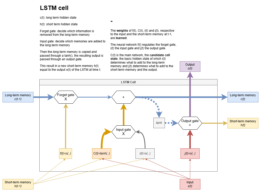
- Long short-term memory (LSTM): most widely used memory cell architecture:
- Preserve gradient from vasinsing allowing theam to learn long-term dependencies.
- Effective for sequential data operations. Excel in:
- time series prediction,
- speech recognition,
- natural language processing.
- Cell state: memory of the network that stores long-term information in a long short-term memory (LSTM) cell.
- Gates: mechanism used by memory cells to control what information to store They are Sigmoid-activated units that control the flow of information in a long short-term memory (LSTM) cell.
- Forget gate: decides which information to discard from the LSTM cell state: \(f_t=\sigma(W_f[h_{t-1},x_t]+b_f)\)
- Input gate: decides which new information to add to the LSTM cell state: \(i_t=\sigma(W_i[h_{t-1},x_t]+b_i)\)
- Candidate cell state: suggests new information to add to the LSTM cell state: \(\tilde{C_t}=\tanh(W_C[h_{t-1},x_t]+b_C)\) where \(C_t\) is the cell state.
- Output gate: decides what information to output in the LSTM cell: \(o_t=\sigma(W_o[h_{t-1},x_t]+b_o)\)
LSTM cell state update
The new cell state combines the old state (filtered by the forget gate) and the candidate state (regulated by the input gate):
\(C_t=multiply(f_t,C_{t-1})+multiply(i_t,\tilde{C_t})\)
Where:
- \(C_t\): cell state
- \(f_t\): forget gate
- \(i_t\): input gate
- \(\tilde{C_t}\): candidate cell state.
Hidden state is updated with element-wisde multiplication of output gate and cell state:
\(h_t=multiply(o_t,tanh(C_t))\)
Where:
- \(h_t\): hidden state
- \(o_t\): output gate
- \(tanh(C_t)\): maps the cell state to a bounded range -1,1.
The goal of mapping the cell state to a bounded range -1,1 is to allow non-linear transformations, making it suitable for tasks like sequence modeling and memory representation.
In LSTM, the output of each gate is a matrix of weights in range 0,1 which are multplied element-wise with the relevant tensors to modulate flow of information.
Applications:
- Time series forecasting (e.g. predicting stock prices).
- Task involving long-term dependencies in sequential data, like machine translation.
Limitations:
- RNNs and LSTMs cannot be effectively applied to image classifications tasks, since data is not sequential.
Generative Adversarial Networks
Generative Adversarial Networks (GANs) are a class of machine learning models that are widely used for generating new data that closely resembles a given dataset. They were introduced by Ian Goodfellow and his collaborators in 2014.
GANs consist of two neural networks:
-
Generator (G):
- The generator's role is to create fake data (e.g., images) that is as realistic as possible. It takes random noise (typically from a uniform distribution) as input and transform it into data that resembles the training data.
-
Discriminator (D):
- The discriminator's role is to distinguish between real data (from the training set) and fake data (produced by the generator). It outputs a probability indicating whether a given input is real or fake.
These two networks are trained simultaneously in a zero-sum game:
- The generator tries to "fool" the discriminator by producing increasingly realistic data.
- The discriminator tries to improve its ability to detect fake data.
The competition between these two networks drives both to improve over time.
Objective function. The goal of the GAN is to optimize the following minimax game:
\(\min_G \max_D \mathbb{E}_{x \sim p_\text{data}(x)}[\log D(x)] + \mathbb{E}_{z \sim p_z(z)}[\log(1 - D(G(z)))]\)
- \(p_\text{data}(x)\): Real data distribution
- \(p_z(z)\): Noise distribution
- \(D(x)\): Probability that \(x\) is real
- \(G(z)\): Generated data
The generator minimizes the probability of the discriminator correctly identifying fake data, while the discriminator maximizes its classification accuracy.
Applications:
- Image generatrion
- Create realistic images from noise (e.g., DeepArt, image synthesis).
- Super-resolution:
- Enhance image resolution (e.g., SRGAN).
Mode Collapse
The generator learns to output samples from only a few of the classes present in the training data (example of digits 0-9: use always 1 or 7 because are similar).
Latent space
Once a GAN has successfully been trained, we can discard the discriminator and use the generator to create new samples. We do this simply by feeding it any input vector from the same noise distribution we drew from during training. The space from which we sample these vectors is called the latent space.
One fascinating aspect of GANs is that we can often perform highly interpretable arith metic on vectors sampled from the latent space. For example, consider a GAN trained to generate images of faces. Experiments, such as those performed by Radford et al. (2015), show that, if \(G(z^(1))\) depicts a woman with glasses, \(G(z^2)\) depicts a woman without glasses and \(G(z^3)\) depicts a man without glasses, then \(G(z^1) − G(z^2) + G(z^3)\) is an image of a man with glasses.
We can also use the latent space to interpolate between different generator outputs. For example, if we depict the output obtained by sampling along the line between two latent vectors, it results in a smooth deformation from one face to another.
Conditional GAN (cGAN)
Conditional GANs (cGANs) are a type of Generative Adversarial Network (GAN) that introduce conditioning variables to guide the data generation process. Unlike traditional GANs, which generate data without any control over the output, cGANs allow for the generation of specific types of data based on additional input information.
In cGANs, both the generator and the discriminator are conditioned on auxiliary information \(y\), which could be:
- Class labels (e.g., "cat" or "dog").
- Text descriptions (e.g., "a red car").
- Any other data (e.g., segmentation maps, images).
The generator take as input a random noise vector \(z\) and the condition \(y\), and generates data \(G(z, y)\).
The discriminator receives both real or fake data and the condition \(y\), and learns to determine if the data corresponds to the given condition.
The objective function for cGANs is modified to incorporate the conditioning variable \(y\):
\(\min_G \max_D = \mathbb{E}_{x \sim p_\text{data}(x)}[\log D(x, y)] + \mathbb{E}_{z \sim p_z(z)}[\log(1 - D(G(z, y), y))]\)
Autoencoders
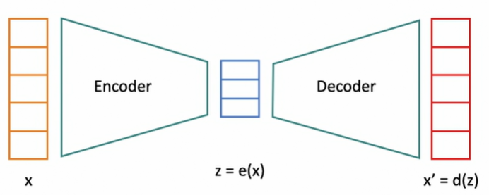
Autoencoders are neural networks whose superficial task is to learn the identity function \(fx=x\). In other words, autoencoders learn to reconstruct their input. The real purpose of the autoencoder, however, is to learn an efficient representation of the input data that, ideally, preserves only the information required to obtain a sufficiently faithful reconstruction.
Consider, for example, a data set of images of a fixed size consisting of a single solid color. Supposing we know the size of the images, we only need the three numbers corre sponding to the red, green, blue (RGB) value of the color to reconstruct the image. An autoencoder is capable of learning such a representation for the images. In much more complicated settings, autoencoders are high-level tools for dimensionality reduction, i.e., extraction of the most important features in the input data. Applications include data compression, denoising, and upscaling.
They consist of two main parts:
1. Encoder
- The encoder compresses the input data into a smaller representation called the latent space or bottleneck.
- This is achieved by applying a series of transformations (linear or non-linear) to map the input data to a lower-dimensional space.
-
Mathematically, the encoder can be represented as:
\(z = f(x; \theta)\)
where \(x\) is the input data, \(z\) is the latent representation, and \(\theta\) are the parameters (weights and biases) of the encoder.
2. Decoder
- The decoder reconstructs the input data from the latent space representation.
- It applies transformations to map the compressed data back to the original input space.
-
Mathematically, the decoder can be represented as:
\(\hat{x} = g(z; \phi)\)
where \(z\) is the latent representation, \(\hat{x}\) is the reconstructed data, and \(\phi\) are the parameters of the decoder.
-
Loss Function: The training objective of an autoencoder is to minimize the reconstruction loss, which measures the difference between the input \(x\) and the reconstructed output \(\hat{x}\). Common loss functions include:
- Mean Squared Error (MSE): \(\text{Loss} = \| x - \hat{x} \|^2\)
- Cross-Entropy Loss (for binary or categorical data).
-
Unsupervised Learning: Autoencoders don't require labeled data since the goal is to reconstruct the input itself.
Variants of Autoencoders
-
Denoising Autoencoders (DAE):
- Introduce noise to the input and train the network to reconstruct the original, noise-free data.
- Used for noise reduction and feature learning.
-
Sparse Autoencoders:
- Encourage sparsity in the latent representation by adding a sparsity penalty to the loss function.
- Useful for discovering underlying features of the data.
-
Variational Autoencoders (VAE):
- Probabilistic model that introduces a stochastic element by learning the parameters of a distribution (e.g., mean and variance).
- Often used in generative modeling to produce new samples.
-
Contractive Autoencoders:
- Add a penalty to the loss function to ensure robustness to small changes in the input.
- Focus on learning invariant representations.
-
Convolutional Autoencoders:
- Use convolutional layers instead of fully connected layers, making them suitable for image data.
Applications:
- Dimensionality Reduction: Similar to Principal Component Analysis (PCA), autoencoders can reduce data dimensions while preserving important features.
- Anomaly Detection: Anomalies are harder to reconstruct, so high reconstruction loss can signal outliers.
- Generative Models: Variational Autoencoders can generate new data samples.
- Data Denoising: Clean noisy input data.
- Pretraining: Autoencoders can initialize deep networks by providing a meaningful starting point.
Challanges:
- Overfitting: Autoencoders may memorize the input data rather than learning meaningful representations.
- Hyperparameter Tuning: Choosing the right architecture, latent dimension size, and regularization is critical for good performance.
Parallel training techniques
Direct Feedback Alignment (DFA)
Direct Feedback Alignment is an alternative to backpropagation, aimed at reducing the computational dependency between layers during training. Instead of propagating the error gradients backward through each layer, DFA uses random projections to provide approximate feedback signals directly to each layer.
- Random Feedback Matrix: A fixed, random matrix is used to project the output error directly onto the layers.
- Decoupling: Each layer gets its feedback signal independently, without relying on computations from adjacent layers.
- No Gradient Propagation: Removes the need for calculating exact gradients through the network, which can be computationally intensive.
- Biological Plausibility: Inspired by how biological neural systems might operate, as they lack a clear mechanism resembling backpropagation.
Challanges:
- DFA often underperforms compared to backpropagation in terms of convergence and accuracy.
- Its effectiveness depends on the quality of the random feedback alignment.
Synthetic Gradients
Synthetic Gradients decouple the training of network layers by generating gradients locally for each layer using a learned model rather than backpropagating gradients from the output loss.
- Gradient Model: A small neural network or function approximator predicts the gradients for a given layer, based on local information (e.g., the activations of that layer).
- Parallelism: Enables simultaneous training of layers, as the dependency on the exact gradient computation from the preceding layers is removed.
- Efficiency: Reduces memory usage and computational bottlenecks associated with backpropagation.
Challanges:
- The synthetic gradient model must be trained effectively to match the true gradients; poor approximation can degrade overall performance.
- May add complexity to the model due to the additional gradient prediction network.
Decoupled Neural Interfaces (DNIs)
DNIs use synthetic gradients and/or synthetic inputs to break the computational dependencies ("locking") inherent in standard backpropagation. This allows simultaneous training of different layers or modules in a neural network, improving parallelization.
-
Types of Locking in Backpropagation:
- Forward Locking: A layer must wait for previous layers to compute outputs.
- Update Locking: Weight updates depend on a full forward pass and loss computation.
- Backward Locking: Gradient updates require a complete backward pass through successive layers.
-
Functionality of DNIs:
- Synthetic Gradients: Break backward locking by approximating gradients locally.
- Synthetic Inputs: Break forward locking by providing learned inputs for subsequent layers.
- Combined use of synthetic gradients and inputs eliminates update locking, enabling simultaneous updates across layers.
-
Implementation Example:
- A network with 100 layers is divided into two modules (\(\mathcal{M}_1\) and \(\mathcal{M}_2\)) trained on separate GPUs.
- Synthetic input and gradient models (\(I_{50}\) and \(M_{51}\)) allow each module to operate independently.
-
Training steps:
- Compute synthetic inputs (\(h_{50}\)) via \(I_{50}\).
- Perform forward passes through \(\mathcal{M}_1\) and \(\mathcal{M}_2\).
- Compute synthetic gradients (\(\delta_{51}\)) and true gradients (\(\delta_{100}\)).
- Update weights in each module using their respective gradients.
- Train \(I_{50}\) and \(M_{51}\) using the intermediate results.
-
Advantages:
- Enables parallel training across multiple processors.
- May act as a regularizer, reducing overfitting.
-
Challenges:
- Training the synthetic models requires extra computation, which may offset parallelization gains.
Conditional DNIs (cDNIs)
- Variation of DNIs where the synthetic gradient models (\(M_i\)) take both the hidden activations (\(h_i\)) and the ground-truth labels (\(y\)) as inputs.
- Improves performance by providing additional information, reducing underfitting compared to standard DNIs.
Applications and Practical Use:
- DNIs are used only during training to improve weight computation efficiency. Once training is complete, the network operates with a standard forward pass.
- Effective in modularizing large networks for distributed or multi-GPU environments.
- Useful in regularization and transfer learning contexts, depending on network design and task requirements.
Comparison and Interplay
| Aspect | DFA | Synthetic Gradients | Decoupled Interfaces |
|---|---|---|---|
| Feedback Type | Random, fixed | Learned, adaptive | Interface-driven, local |
| Coupling | Decoupled feedback per layer | Partially decoupled | Fully decoupled |
| Biological Plausibility | Moderate | Low | Low |
| Parallelism | Moderate | High | High |
| Performance | Often suboptimal compared to BP | Can match BP if gradients are accurate | Dependent on interface design |
These approaches focus on reducing the computational challenges of backpropagation and enabling more scalable and biologically inspired training paradigms.
Attention Mechanisms and Bidirectional RNNs
In Neural Machine Translation (NMT)
Bidirectional RNNs
Bidirectional Recurrent Neural Networks (RNNs) process sequential data (e.g., sentences) in both forward and backward directions to capture dependencies from both past and future contexts. Each input word (\(x_t\)) is processed by forward and backward layers, producing an intermediate concatenated vector (\(h_t\)).
Challenges:
- Bidirectional RNNs condense information from the entire sequence into a fixed-dimensional vector, which struggles to handle long sequences effectively.
- Performance decreases for lengthy sentences due to this compression.
Attention Mechanisms
Inspired by human translators, attention mechanisms enable a model to focus on the most relevant parts of an input sequence when generating each part of an output sequence. Proposed by Bahdanau et al. (2014), the idea is to dynamically assign "attention weights" to different parts of the input, which helps in translating long sentences.
Architecture:
-
Encoder-Decoder Model:
- Encoder: Processes the input sequence (\(x\)) to generate contextual representations (\(h_e\)).
- Decoder: Uses the encoder’s outputs and an attention mechanism to produce the translated output sequence (\(y\)).
-
Attention Mechanism Components:
- Attention Vector (\(\alpha_{s,t}\)): Weights determining the importance of the \(t\)-th word in the input for the \(s\)-th word in the output.
- Properties: \(0 \leq \alpha_{s,t} \leq 1\), and \(\sum_t \alpha_{s,t} = 1\).
- Context Vector (\(c_s\)): Weighted sum of encoder outputs, focused on the input segments relevant to the current output word.
- Attention Vector (\(\alpha_{s,t}\)): Weights determining the importance of the \(t\)-th word in the input for the \(s\)-th word in the output.
-
Training Attention:
- Attention weights (\(\alpha_{s,t}\)) are derived from intermediate scores (\(e_{s,t}\)) using a softmax function.
- Scores are computed via a neural network combining encoder outputs (\(h_t^e\)) and decoder states (\(h_{s-1}^d\)).
Advantages:
- Improves performance on long sentences by dynamically selecting relevant information.
- Makes the model more interpretable by highlighting which parts of the input influence specific outputs.
- Has applications beyond NMT, such as image captioning, where attention identifies important image regions for generating descriptive text.
Attention mechanisms have been successfully applied in diverse tasks like image captioning (e.g., Xu et al., 2015) and other sequence-to-sequence problems.
Diffusion Models
Generative Learning Trilemma: A generative model needs to satisfy three requirements for widespread adoption:
- High-Quality Samples: The model should produce samples that are as realistic as possible.
- Fast Generation: The process of generating samples should have low computational complexity, enabling real-time applications.
- Good Diversity (Mode Coverage): The model should capture the diversity of the input data, including rare samples.
Challenges with GANs:
- GANs produce very high-quality samples quickly.
- However, they often lack diversity and do not cover the full range of the input data well.
Diffusion Models:
- Diffusion models can generate high-quality samples with better diversity and mode coverage compared to GANs.
- They are more suitable when a good representation of rare samples is required.
The diffusion model was introduced in the 2020 paper "Denoising Diffusion Probabilistic Models" by Jonathan Ho and colleagues. The original paper did not claim that diffusion models generated better images than GANs. Many papers have since improved upon the original diffusion model, with some claiming that diffusion models now outperform GANs in image synthesis. The authors of the original paper published another paper showing that their improved diffusion model captured the breadth of training data variance better and beat state-of-the-art GANs in image generation tasks.
FID: the quality of images generated by a model is evaluated using the FID (Frechet Inception Distance) score. A lower FID score indicates better image quality, with a perfect score being 0.0.
Comparison with GANs: The improved diffusion model, known as the Ablated Diffusion Model (ADM), achieved the best FID scores across various datasets, outperforming several GANs.
Denoising diffusion probabilistic model (DDPM)
Diffusion Process:
- Starts with a real image from the training dataset.
- Noise is added iteratively in small steps, following a Gaussian distribution.
- After many steps, the image becomes pure noise.
Forward Diffusion Process: Adding noise to an image in incremental steps until it becomes unrecognizable.
Reverse Diffusion Process:
- The goal is to reverse the forward process.
- Start with pure noise and iteratively remove noise to generate an image.
- A neural network is trained to learn this reverse process.
Training Objective: Train a neural network to approximate the reverse diffusion process, enabling the generation of images from noise.
Forward Diffusion Process
- Start with a sample base image \(x_0\) from the input training data.
- Incrementally and iteratively add Gaussian noise to the image.
- At each step \(t\), the image \(x_t\) has more noise added.
- This process continues for \(T\) time steps, resulting in \(x_T\), an image that is pure noise.
- In practice, \(T\) is typically between 1,000 to 4,000 steps.
- The final image \(x_T\) is a Gaussian distribution with mean 0 and variance 1.
The forward diffusion process is modeled as a Markov chain.
- Each step \(t\) depends only on the previous state \(t-1\).
- This means the probability of each event depends only on the previous state.
Formulas:
- State Transition Distribution: \(q(x_t | x_{t-1})\)
- Variance: \(\beta_t\) (variance at different time instances, increases over time but always between 0 and 1)
- this is a hyperparameter.
- Mean: \(\sqrt{1 - \beta_t} \cdot x_{t-1}\)
- This formula ensures that the mean is non-zero as long as \(x_{t-1}\) is non-zero.
- Since \(\beta_t\) is between 0 and 1, \(\sqrt{1 - \beta_t}\) is also between 0 and 1, which scales \(x_{t-1}\) to a value less than or equal to its original magnitude.
- As \(T\) approaches infinity, \(q(x_T | x_0)\) approaches a Gaussian with mean 0 and variance 1.
Reverse Diffusion Process
- Starts with pure noise, represented by \(x_T\).
- Generates an image similar to those in the training data by reversing the noise addition process.
- Modeled as a Markov chain, where each state depends only on the previous state.
Neural Network:
- Learns the parameters of the transition in the reverse process.
- Objective is to learn the mean and variance of the denoising process to generate images from noise.
Formulas:
- Reverse Transition: \(p_\theta\)
- Given an image at time \(t\) (\(x_t\)), the goal is to get to \(x_{t-1}\).
- Each reverse transition is a Gaussian with a certain mean and variance.
- The mean and variance depend on the sample \(x_t\) and the forward diffusion process variance schedule (\(\beta_t\)).
\(p_\theta(x_{t-1} \mid x_t) = \mathcal{N}\left(x_{t-1}; \color{red}{\mu_\theta(x_t, t)},\, \color{red}{\Sigma_\theta(x_t, t)}\right)\)
The neural network learns to undo the noise added at each time step. Noise was added incrementally and iteratively in the forward process, allowing the reverse process to function effectively.
Training Diffusion Models
- Uses a neural network to approximate the reverse diffusion process.
- The reverse diffusion process has the same functional form as the forward diffusion process.
- The model learns the parameters to generate images from noise.
The diffusion model can be thought of as a latent variable generator model, similar to a Variational Autoencoder (VAE).
Simple Autoencoders:
- Used for dimensionality reduction.
- Extract latent features from input data.
- Encode input images into lower dimensionality.
- Decoder regenerates the original input from latent features.
Variational Autoencoders (VAEs):
- Probabilistic in nature.
- Output is not deterministic but probabilistic.
- Encoder produces a distribution over a latent variable \(z\).
- Decoder generates data that looks like the input from the latent sample.
Relation to Diffusion Models:
- The forward diffusion process is similar to the encoder in a VAE.
- The reverse diffusion process is similar to the decoder in a VAE.
- But in diffusion models, forward process is fixed and involves adding noise in a specific way.
- Only the neural network for the reverse process needs to be trained.