
This study was carried out as appendix of a research assignment at IU University of Applied Sciences, in 2025, to complement the theoretical foundations discussed. The objective was to design and analyze an original experimental case study, drawing inspiration from major milestone techniques in reinforcement learning-based neural architecture search (NAS) for automation. The foundational approaches explored in this work are detailed in the following key literature:
- Baker et al. (2017): MetaQNN: A reinforcement learning approach for automated neural architecture design.
- Zoph & Le (2017): Neural Architecture Search with Reinforcement Learning.
- Zoph et al. (2018): Learning Transferable Architectures for Scalable Image Recognition.
Full code can be found at the following GitHub repository: DLMAIRIL_RL_based_NAS.
About the Proposed Case Study
The implementation was carried out using Python 3.9 to ensure compatibility with TensorFlow and the AWS training jobs images. For this academic assignment, a custom benchmark dataset was created rather than relying on standard datasets, allowing for a more thorough demonstration of both theoretical concepts and practical skills in Reinforcement Learning and Neural Architecture Search.
The custom dataset was inspired by a hypothetical IoT application: a garden robot designed to autonomously collect leaves using an integrated vacuum system. The robot's AI must reliably distinguish leaves from other types of ground cover to perform its task.
For this assignment, the dataset was synthetically generated using a Python script with the PIL library. It contains 4,000 images (total size: 12.8 MB, uploaded to AWS S3), depicting leaves and diverse grounds to create challenging scenarios for the recognition algorithm. Images are 64x64 pixels, allowing for controlled experiments with deeper CNN architectures in a binary image classification setting.
Below are examples illustrating the dataset, showing typical leaf samples and challenging background scenarios used for model training.
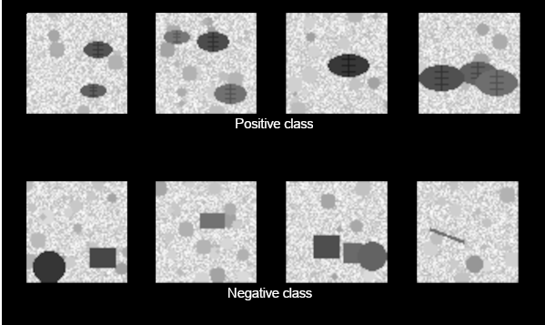
Sample images from the custom leaves dataset: examples with and without leaves.
Model training was performed using AWS machine learning services as part of the study project for the Machine Learning Specialty certification. Amazon SageMaker provided the necessary GPU resources for model training, while Amazon S3 was used to store both the dataset and experiment results.
Implementation Summary: MetaQNN Approach from Baker et al. (2017)
Due to computational constraints, even with GPU acceleration, the implementation complexity was limited. Fewer models were trained for each epsilon value compared to the original MetaQNN setup, and each model was trained for fewer epochs. Early stopping was applied to terminate poorly performing architectures sooner. These adaptations were necessary to ensure the experiments could be completed within practical time and hardware limits.
The implementation was carried out using standard Python, without relying on external reinforcement learning libraries. This direct approach was chosen because updating the \(Q\)-table in a discrete action space is straightforward and does not require advanced RL frameworks. By avoiding abstraction layers, the algorithm's internal dynamics and learning process remain fully exposed and transparent, providing a more comprehensive and accessible understanding of how \(Q\)-learning operates in the context of neural architecture search.
The full source code is available in the associated GitHub repository: https://github.com/michelesalvucci/DLMAIRIL_RL_based_NAS.
Implementation Details
The core \(Q\)-learning algorithm follows Baker et al.'s specifications closely:
# Q-learning parameters from Baker et al. (2017, p. 5)
Q_LEARNING_RATE = 0.01  # Learning rate for Q-updates
DISCOUNT_FACTOR = 1     # No discounting for finite horizon problem
DEFAULT_Q_VALUE = 0.5   # Initial Q-value for unexplored state-action pairs
LAYERS_DEPTH_LIMIT = 12 # As per Baker et al. (2017) - Maximum depth of the architecture

# Architectures training parameter
IMG_SIZE = (64, 64)
LEARNING_RATE = 0.001  # Learning rate for the optimizer
EPOCHS = 15 # Number of epochs for training, Baker et al. (2017, p. 6) uses 20 epochs, here I use 15 for quicker testing
BATCH_SIZE = 128
The \(Q\)-update follows the standard formula from Equation 3 in Baker et al.:
def __update_q_values(self, architecture: List[AbstractLayer], reward: float):
    # ... state processing ...
    self.q_table[state_key][action] = ((1 - Q_LEARNING_RATE) * Q_s1_a + Q_LEARNING_RATE * (reward + DISCOUNT_FACTOR * max_Q_s2))
Experience Replay implementation: following Baker et al.'s approach of sampling \(n\) models from experience replay.
def update_with_experience_replay(self, architecture: List[AbstractLayer], reward: float):
    self.replay_memory.add_experience(architecture, reward)
    # Sample batch and update Q-values for better learning stability
    if self.replay_memory.size() >= SAMPLED_MODELS_FROM_EXPERIENCE_REPLAY:
        batch = self.replay_memory.sample_batch(SAMPLED_MODELS_FROM_EXPERIENCE_REPLAY)
        for experience in batch:
            self.__update_q_values(experience['architecture'], experience['reward'])
Layer Constraints and Valid Actions: the implementation strictly follows Baker et al.'s layer constraints.
def __get_valid_actions(self, state: AbstractLayer, current_r_size: float):
    next_layer_depth = state.layer_depth + 1 if state is not None else 0
    r_size_bin = get_representation_size_bin(current_r_size)
    # Based on Baker et al. (2017, p. 5)
    available_layers = ['C', 'P', 'FC', 'GAP', 'SM']
    if state is not None:
        if next_layer_depth == LAYERS_DEPTH_LIMIT:
            available_layers = ['SM'] if state.type == 'FC' else ['GAP', 'SM']
        else:
            if state.type == 'FC':
                available_layers = ['FC', 'SM']
            if state.type == 'P' and 'P' in available_layers:
                available_layers.remove('P')
            if (self.fc_layers_selected >= 2 or current_r_size > 8) and 'FC' in available_layers:
                available_layers.remove('FC')

    # Parameters according to the table in  Baker et al. (2017, p. 5)
    if 'C' in available_layers:
        for receptive_field_size in [1, 3, 5]:
            # Representation size constraint: receptive field size <= current r_size
            if receptive_field_size <= current_r_size:
                for receptive_field in [64, 128, 256, 521]:
    ...
Architecture building process: the CNN builder translates abstract layer representations into Keras models.
def build_cnn(architecture: List[AbstractLayer]) -> Sequential:
    ...
    for i, layer in enumerate(architecture):
        if isinstance(layer, ConvolutionalLayer):
            conv_layer = Conv2D(filters=layer.receptive_fields, kernel_size=layer.field_size, strides=layer.stride, ... )
            model.add(conv_layer)
        elif isinstance(layer, PoolingLayer):
            pooling_layer = MaxPooling2D(...)
            ...
        if not isinstance(layer, SoftmaxLayer) and (i + 1) % 2 == 0:
            dropout_count += 1
            dropout_prob = dropout_count / (2 * total_dropout_layers) if total_dropout_layers > 0 else 0
            model.add(Dropout(dropout_prob))
Epsilon-Greedy exploration schedule: following Baker et al.'s exploration strategy with decreasing epsilon values, but using halved values to accommodate computational constraints.
EPSILON_TO_NUM_MODELS_MAP = {
    1.0: 750,  # High exploration initially
...
    0.1: 150    # Low exploration in final stages
}

for epsilon, num_models in EPSILON_TO_NUM_MODELS_MAP.items():
    for _ in range(num_models):
        # episode

def __choose_action(self, state: AbstractLayer, current_r_size: float) -> AbstractLayer:
    #Epsilon-greedy action selection
    ...
    if random.random() < self.epsilon:
        return random.choice(valid_actions)  # Exploration
    else:
        return self.__get_best_action(valid_actions, state_key) # Exploitation: choose action with highest Q-value
Training and results
Training was performed on an AWS SageMaker training job using a NVIDIA A10G Tensor Core GPU (ml.g5.xlarge) instance. The full search process required approximately 2 hours. Due to computational constraints, each candidate model was trained for only 15 epochs during the search phase, with a validation set comprising 20% of the dataset. The total number of models explored (search space) was reduced to one-tenth of the original MetaQNN paper, and the number of sampled models from experience replay was scaled accordingly. Early stopping was used to halt training of underperforming architectures, further reducing computation time. The custom leaves dataset described in the introduction was used throughout to maintain consistency with the other experiment.
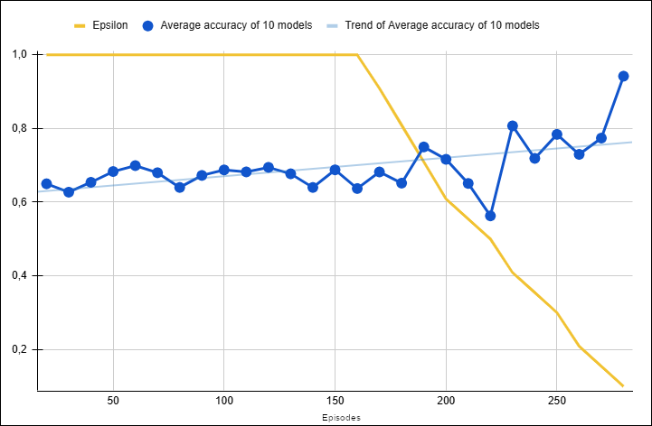
Figure: Average validation accuracy progression during MetaQNN-based NAS on the custom leaves dataset (averaged over 10-model intervals).
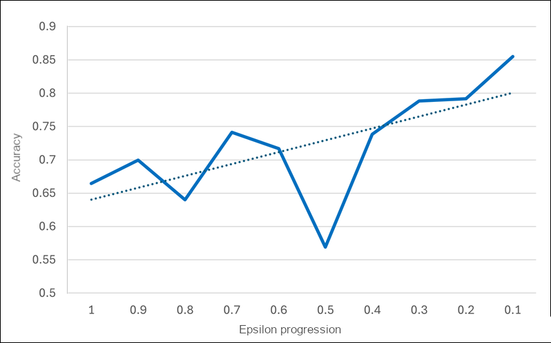
Figure: Mean reward for each epsilon value in the MetaQNN-based case study custom search.
The results, as shown in the plots, indicate that decreasing \(\epsilon\) led to improved model accuracy. Initially, with \(\epsilon=1\), the agent selected architectures randomly, resulting in many models predicting the majority class and achieving around 50% accuracy. As \(\epsilon\) decreased, the agent shifted from exploration to exploiting better architectures, which increased validation accuracy and reduced the number of constant predictors. Although the number of models explored was limited, the mean reward (validation accuracy) generally increased as \(\epsilon\) decreased.
The top 10 performing architectures identified during the search were then fine-tuned: each was retrained for twice as many epochs and evaluated on the test set (30% of the dataset).
The highest validation accuracy achieved by the discovered architectures was 98.5% (architecture: P(2,2) - C(256,5,1) - C(128,1,1) - P(3,2) - C(64,3,1) - C(521,5,1) - C(128,3,1) - C(64,3,1) - P(3,3) - SM()). Average test accuracy of the top 5 was 90.7%. The table below summarizes the top 5 architectures found, including their parameter counts and test set accuracies:
| Rank | Architecture | # Parameters | Test Accuracy (%) |
|---|---|---|---|
| 1 | P(2,2) - C(256,5,1) - C(128,1,1) - P(3,2) - C(64,3,1) - C(521,5,1) - C(128,3,1) - C(64,3,1) - P(3,3) - SM() | 1,623,882 | 98.50 |
| 2 | C(128,5,1) - C(256,5,1) - C(256,5,1) - SM() | 3,383,041 | 96.92 |
| 3 | C(256,1,1) - C(521,5,1) - C(64,5,1) - P(5,3) - C(128,5,1) - P(2,3) - C(521,3,1) - P(5,2) - C(64,1,1) - SM() | 5,009,171 | 92.50 |
| 4 | C(128,5,1) - C(64,1,1) - SM() | 241,985 | 83.25 |
| 5 | C(128,3,1) - C(128,1,1) - SM() | 509,825 | 83.08 |
Top-performing architectures discovered using the MetaQNN method in the custom case study, including parameter counts and corresponding test set accuracies.
From the progression of architectures accuracy as \(\epsilon\) decreases, a clear pattern emerges: numerous architectures achieve exactly 50.535% accuracy, which corresponds to the majority class baseline of the validation set. This occurs because poorly performing architectures tend to default to predicting the most frequent class. In contrast, models that successfully learn meaningful features achieve significantly higher accuracies, typically jumping to 75% or above. This creates a bimodal distribution between "constant predictors" and "successful models". As \(\epsilon\) decreases (meaning less exploration and more exploitation), the frequency of these baseline-performing models diminishes.
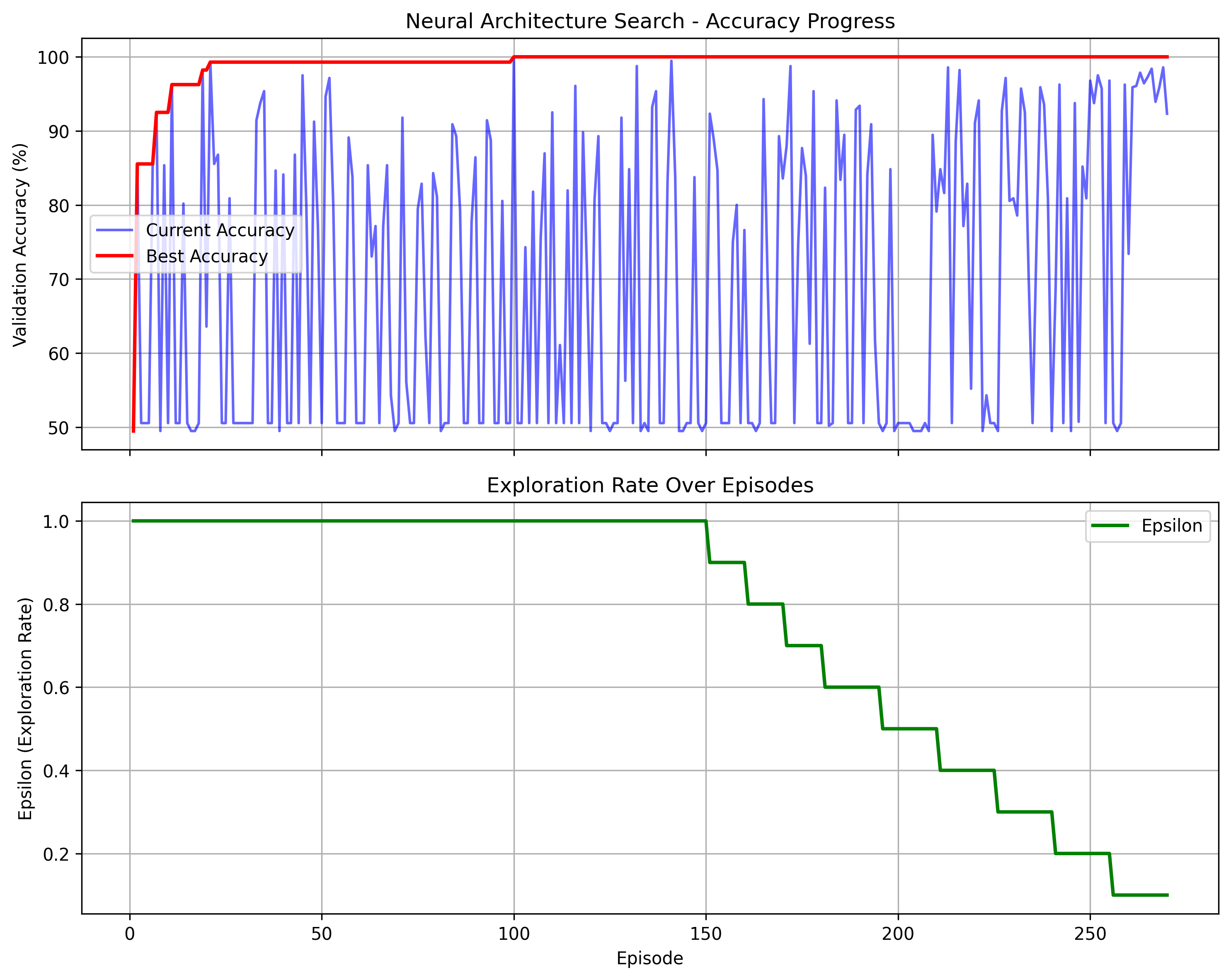
Progression of architectures as epsilon decreases on the custom leaves dataset.
Overall, the MetaQNN approach shows that \(Q\)-learning can automate CNN architecture design effectively, even with computational constraints. However, the resource demands of early RL-based NAS methods highlight the need for more efficient and transferable strategies, which are discussed in the next section.
Implementation Summary: NASNet architecture from Zoph et al. (2018)
nas_net_architecture experimental module (see GitHub source code) implements a NAS framework inspired by the approaches described Zoph and Le, 2017, Neural Architecture Search with Reinforcement Learning and in Zoph et al. 2018, Learning Transferable Architectures for Scalable Image Recognition.
The project was implemented in Python 3.9 and trained using AWS SageMaker, as outlined in the introduction. To address computational limitations, both the search space and the number of training episodes were reduced. This enabled experimentation on the actual leaves dataset, but limited the statistical significance of the results. To address such computational constraints, the mock_train_and_evaluate_child_network() function was implemented. This function produces a non-linear reward based on specific architectural features, prioritizing certain cell types. This approach enabled fast experimentation and analysis of agent learning behavior over hundreds of episodes, even when running on a CPU-only local environment.
RNN Controller
The controller in this code is trained using the REINFORCE policy gradient method. It samples actions (architecture decisions) and receives a reward based on the performance of the generated child network on the validation data.
To reduce variance in policy updates, a moving baseline was used, similar to the baseline technique in the original paper. The baseline is computed as a combination of recent and historical rewards, and the difference between the reward and the baseline is used to update the controller.
def train_step(self):
    # RNN Controller code
    ...
    # Use the highest of these to prevent baseline from dropping too much
    baseline = max(recent_mean, historical_mean, best_baseline)
    ...
    # Difference = reward - baseline (positive for good episodes)
    difference = final_reward - baseline
    ...
    # REINFORCE loss: -log(prob) * difference
    # Policy gradient update: theta = theta + alpha * E[pi_theta](s, a) * (R_k - b)
    # tf.reduce_mean computes the expected value
    # 'difference' represents (R_k - b), i.e., reward minus baseline
    # Negative sign: Minimizing this loss (as done by optimizers like Adam) is equivalent to maximizing the objective (gradient ascent), since the objective is negated.
    loss = -tf.reduce_mean(tf.math.log(selected_action_probs) * differences)
    # Compute and apply gradients of the loss with respect to parameters
    gradients = tape.gradient(loss, self.policy_net.trainable_variables)
    self.optimizer.apply_gradients(zip(gradients, self.policy_net.trainable_variables))
Unlike \(Q\)-learning, policy gradient methods do not use \(\epsilon\)-greedy exploration. Instead, actions are sampled directly from the softmax probabilities (Sutton and Barto, 2018, pp. 322–324). This can lead to premature overconfidence if early rewards or initial weights bias the controller toward certain actions, reducing exploration. To address this, a softmax temperature parameter was introduced, allowing controlled exploration by adjusting the sharpness of the action distribution during sampling.
# Convert "back" probabilities to logits before applying temperature scaling, since softmax uses exp(logits)
logits = tf.math.log(action_probs) / self.temperature
# Action selection based on probabilities of the softmax distribution
action = tf.random.categorical(tf.expand_dims(logits, 0), 1)[0, 0]

def _anneal_temperature(self):
    self.episode_count += 1
    self.temperature = max(
        self.temperature_min,
        self.temperature * self.temperature_decay
    )
Cell Entity and Transfer Learning
The concept of a cell as a modular, transferable building block is adopted from Zoph et al. (2018). The controller predicts the structure of two types of cells (normal and reduction), which are then stacked to form the final network.
The code is structured to allow transferability of discovered cells to larger networks or different datasets, following the transfer learning principles in the 2018 paper. The controller would be trained on a subset comprising 20% of the full leaves dataset, where the validation data is 11% as in Zoph and Le (2017).
val_split_idx = int(0.89 * len(X_trainval)) # Zoph and Le selected 11% of training data for validation
X_train, X_val = X_trainval[:val_split_idx], X_trainval[val_split_idx:]
y_train, y_val = y_trainval[:val_split_idx], y_trainval[val_split_idx:]
SEARCH_DATASET_FRACTION = 0.2 # Use 20% of the data for fast search
trainer = Trainer(fraction=SEARCH_DATASET_FRACTION)
# ... use trainer.mock_train_and_evaluate_child_network() or trainer.train_and_evaluate_child_network() ...After the search, the top 10 architectures are retrained on the full dataset for final evaluation:
from trainer import Trainer
from cnn_builder import build_child_network

# Assume sorted_cells is a list of (architecture_str, reward) tuples
trainer = Trainer(fraction=1.0)  # Use the full dataset
for i, (cell_str, _) in enumerate(sorted_cells[:10]):
    ...
    model = build_child_network(normal_cell, reduction_cell, B=2)
    trainer.train_and_evaluate_child_network(model)
Mock deterministic reward function
The reward function is designed to simulate the evaluation of an architecture generated by the controller by examining the sequence of actions selected by the agent. Each set of five actions represents a block in the architecture, with specific indices corresponding to input selections, operation types, and combination strategies. This structure follows the conventions described by Zoph et al. (2018, p. 3), where these action steps map to stages in the agent's trajectory. The function first separates the actions into three categories: input actions, operation actions, and combine actions.
The operation actions are analyzed to determine how many are "high" (greater than 8) and "low" (less than 4), which influences the reward calculation. The diversity of input actions and combination strategies is measured by counting the number of unique values and normalizing by the possible range, encouraging architectures that use a variety of connections and combination methods. The reward calculation starts with a base value and adds bonuses for a high ratio of complex operations, diversity in operations, input variety, and combination strategy variety. There is also a small penalty for using too many simple operations. Additionally, a non-linear bonus is applied based on the mean of the operation actions, introducing more variation into the reward.
Finally, the computed reward is clamped to ensure it stays within a reasonable range (between 0.5, the binary classification baseline, and 0.998), preventing extreme values. This function is useful for quickly estimating the "quality" of a proposed architecture in a reinforcement learning or neural architecture search context, without actually training the network.
Results
Zoph et al. (2018, p. 4) showed that their NASNet cell-based search on CIFAR-10 achieved a 7x speedup over the original REINFORCE-based NAS, cutting search time from 28 to 4 days and improving accuracy. For this assignment, due to computational constraints, I adapted the approach to the custom leaves dataset and evaluated the agent using the mock deterministic reward function described above.
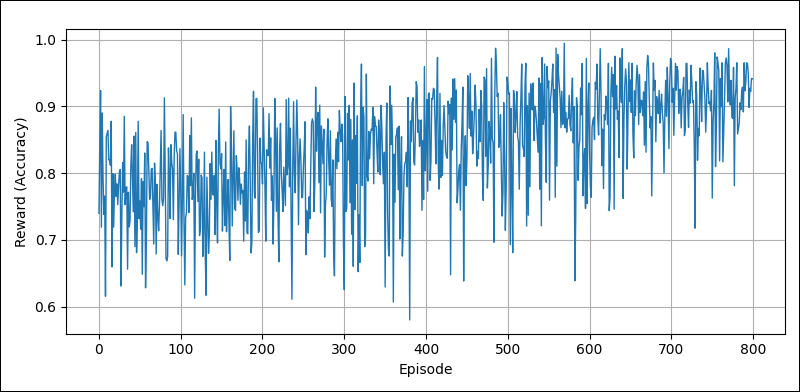
Reward progression of the NASNet RNN controller agent during search for increasingly complex cell architectures, as evaluated by the deterministic mock reward function.
The plot illustrates the training progress of the RNN controller agent using the mock reward function. Across 800 REINFORCE episodes, with a moving baseline and annealing softmax temperature to manage exploration, the agent's average reward steadily increases. Simultaneously, the occurrence of low-reward architectures declines. This indicates that the agent is successfully learning to generate more sophisticated, higher-reward architectures while efficiently navigating the large combinatorial search space.
Bibliography
- Baker, B., Gupta, O., Naik, N., & Raskar, R. (2017). Designing Neural Network Architectures using Reinforcement Learning (No. arXiv:1611.02167). arXiv. https://doi.org/10.48550/arXiv.1611.02167
- Zoph, B., & Le, Q. V. (2017). Neural Architecture Search with Reinforcement Learning (No. arXiv:1611.01578). arXiv. https://doi.org/10.48550/arXiv.1611.01578
- Zoph, B., Vasudevan, V., Shlens, J., & Le, Q. V. (2018). Learning Transferable Architectures for Scalable Image Recognition (No. arXiv:1707.07012). arXiv. https://doi.org/10.48550/arXiv.1707.07012