
This type of analysis can help to develop competitive schemes without weaknesses, that is, they do not expose fixed pre-built strategies that allow you to circumvent the logic coming to the end result without depending on the results of other players.
A ML model can be trained to predict the right strategy based on the strategies of other players.
import pandas as pd
Description
The player should decide how many Coins \(m \in \mathbb{N}^+\) collect in each level of the game. For each collected coin there is a time consumption that will slow down the player on reaching and cross the portal to the next level.
Having:
- \(L_n\): length of the standard level (a level constant)
- \(V\): velocity, the number of previously collected coins given by \(\sum_{1}^{n-1} m_n\)
- \(m_n\): collected coins inside the ongoing level \(n\)
- \(f\): gamer skill factor on moving the player, it is assumed that it affects the result between 3 and 22% (computer will represent it by generating a randomic float between 0.78 an 0.97).
The time \(T\) for reaching the next level \(n+1\) portal is given by:
\($T_n = (L_n - \frac{V}{3} + m_n) f\)$
"""Based on the formula"""

import random

def calculate_T_n(L_n: int, V: int, m_n: int) -> float:
    return round((L_n - (V / 3.00) + m_n) * random.uniform(0.780, 0.970), 3)
Randomic model and dataset construction example
Let's do the very first example by constructing a set of only 4 levels (finally they will be 24 divided in 3 sections).
We are at the first iteraction and the model hasn't got data to understand how many coins collect, so it will go random.
Suppose that level 1 has max 10 \(m\) collectable and a length of \(L_1 = 10\).
At level 1 I collect (randomly) 3 \(m\)s
So, the travel time of the level 1 is:
\(T_1 = L_1 - \frac{V}{3} + m_1 = 10 - \frac{0}{3} + 3 = 13\)
Passing at level 2, where max \(m\)s are 10 and length of \(L_2 = 14\).
At level 2 I collect (randomly) 6 \(m\)
So, the travel time of the level 2 is:
\(T_2 = 14 - \frac{3}{3} + 6 = 19\)
Passing at level 3, where max \(m\)s are 10 and length of \(L_3 = 19\).
At level 3 I collect (randomly ) 1 \(m\)
So, the travel time of the level 3 is:
\(T_3 = 19 - \frac{9}{3} + 1 = 17\)
So, we go for level 4, where length is of \(L_4 = 24\). Here there are no coins to collect, as it is conclusive.
The travel time of the level 4 is:
\(T_4 = 24 - \frac{10}{3} = 20,66\)
We can complete the first row of the dataset from the first random iteration:
| Iteration | \(T_1\) | \(T_2\) | \(T_3\) | \(T_4\) | \(m_1\) | \(m_2\) | \(m_3\) |
|---|---|---|---|---|---|---|---|
| 1 | 13 | 19 | 17 | 20,66 | 3 | 6 | 1 |
So far, data are telling us nothing, but another iteration will be repeated randomly to compare the scorings, and so on there will be several of it. It's important to rimember that the Machine will have to do the best to qualify at each level, even if this could mean to get a low positioning in some level (depending on the number of qualified for each level). It's not signifcant, instead, the total sum of \(T\) performed in all the levels.
import numpy as np

np_dataframe = np.eye(1, 8)
np_dataframe
array([[1., 0., 0., 0., 0., 0., 0., 0.]])np_dataframe[0] = [1, 13, 19, 17, 20.66, 3, 6, 1]
np_dataframearray([[ 1. , 13. , 19. , 17. , 20.66, 3. , 6. , 1. ]])Function for generate an iteration (optionally supplying the randomic \(m_n\)).
from typing import List

def generate_iteration(L_1=10, L_2=14, L_3=19, L_4=24, m_1=None, m_2=None, m_3=None) -> List[float]:
    total_ms: int = 0

    m_1 = m_1 if m_1 else random.randint(0, 10)
    T_1 = calculate_T_n(L_1, total_ms, m_1)
    total_ms += m_1

    m_2 = m_2 if m_2 else random.randint(0, 10)
    T_2 = calculate_T_n(L_2, total_ms, m_2)
    total_ms += m_2

    m_3 = m_3 if m_3 else random.randint(0, 10)
    T_3 = calculate_T_n(L_3, total_ms, m_3)
    total_ms += m_3

    T_4 = calculate_T_n(L_4, total_ms, 0)

    return [T_1, T_2, T_3, T_4, m_1, m_2, m_3]
From the second random iteration emerges:
| Addestramento | \(T_1\) | \(T_2\) | \(T_3\) | \(T_4\) | \(m_1\) | \(m_2\) | \(m_3\) |
|---|---|---|---|---|---|---|---|
| 1 | 13 | 19 | 17 | 20,66 | 3 | 6 | 1 |
| 2 | 17 | 11,66 | 21,66 | 20 | 7 | 0 | 5 |
iteration: int = len(np_dataframe) + 1
np_dataframe = np.append(np_dataframe, [iteration] + generate_iteration(m_1=7, m_2=0, m_3=5))
np_dataframe = np_dataframe.reshape(iteration, 8)
np_dataframe
array([[ 1. , 13. , 19. , 17. , 20.66 , 3. , 6. , 1. ],
[ 2. , 13.317, 17.55 , 16.585, 13.787, 7. , 10. , 5. ]])by looking at the collected \(m\) at the second random iteration we have a better score at level 2 and 4, but a worst score at level 1 and 3. So the iteration 1 and the iteration 2 have both a best score counting (\(Best\)) of 2.
Si prova una terza iterazione:
| Addestramento | \(T_1\) | \(T_2\) | \(T_3\) | \(T_4\) | \(m_1\) | \(m_2\) | \(m_3\) | \(Best\) | |
|---|---|---|---|---|---|---|---|---|---|
| 1 | 13 | 19 | 17 | 20,66 | 3 | 6 | 1 | 2 | |
| 2 | 17 | 11,66 | 21,66 | 20 | 7 | 0 | 5 | 1 | |
| 3 | 16 | 21 | 17 | 18 | 6 | 9 | 3 | 2 |
It's already understanable that iteration 2 strategy is less efficient than 1's and 3's.
iteration: int = len(np_dataframe) + 1
np_dataframe = np.append(np_dataframe, [iteration] + generate_iteration(m_1=6, m_2=9, m_3=3))
np_dataframe = np_dataframe.reshape(iteration, 8)
np_dataframe
array([[ 1. , 13. , 19. , 17. , 20.66 , 3. , 6. , 1. ],
[ 2. , 13.317, 17.55 , 16.585, 13.787, 7. , 10. , 5. ],
[ 3. , 13.659, 18.433, 15.622, 15.464, 6. , 9. , 3. ]])Let's see a fourth, fifth and sixth random iteration:
| Iteration | \(T_1\) | \(T_2\) | \(T_3\) | \(T_4\) | \(m_1\) | \(m_2\) | \(m_3\) | \(Best\) | |
|---|---|---|---|---|---|---|---|---|---|
| 1 | 13 | 19 | 17 | 20,66 | 3 | 6 | 1 | 1 | |
| 2 | 17 | 11,66 | 21,66 | 20 | 7 | 0 | 5 | 1 | |
| 3 | 16 | 21 | 17 | 18 | 6 | 9 | 3 | 2 | |
| 4 | 15 | 14,33 | 25 | 19 | 5 | 2 | 8 | 0 | |
| 5 | 12 | 19,33 | 20,33 | 20 | 2 | 6 | 4 | 1 | |
| 6 | 15 | 17,33 | 20,66 | 19 | 5 | 5 | 5 | 0 |
The strategies of the fourth and of the sixth iteration seem very efficient, but they are never the best in any level, while the best one would seem to be the third. But..
Instead of look a the best score, we suppose that in order to be qualified to the next level is necessary to be in the top two, so \(Qual\) represents the number of times that the iteration would qualify:
| Iteration | \(T_1\) | \(T_2\) | \(T_3\) | \(T_4\) | \(m_1\) | \(m_2\) | \(m_3\) | \(Qual\) | |
|---|---|---|---|---|---|---|---|---|---|
| 1 | 13 | 19 | 17 | 20,66 | 3 | 6 | 1 | 2 | |
| 2 | 17 | 11,66 | 21,66 | 20 | 7 | 0 | 5 | 1 | |
| 3 | 16 | 21 | 17 | 18 | 6 | 9 | 3 | 2 | |
| 4 | 15 | 14,33 | 25 | 19 [pari] | 5 | 2 | 8 | 2 | |
| 5 | 12 | 19,33 | 20,33 | 20 | 2 | 6 | 4 | 1 | |
| 6 | 15 | 17,33 | 20,66 | 19 [pari] | 5 | 5 | 5 | 1 |
Pradoxically, it seems the fourth iteration adopted the best strategy, toghether with the nr 3 and the nr1. But...
Following sequenciality, supposing therefore that for each level there is one eliminated, and at level 3 there are two (as, with different values, will be the final game), we would have the following race:
| Iteration | \(T_1\) | \(T_2\) | \(T_3\) | \(T_4\) | \(m_1\) | \(m_2\) | \(m_3\) |
|---|---|---|---|---|---|---|---|
| 1 | 13 | 19 | 17 | 20,66 | 3 | 6 | 1 |
| 2 | 17 | - | - | - | 7 | - | - |
| 3 | 16 | 21 | - | - | 6 | 9 | - |
| 4 | 15 | 14,33 | 25 | - | 5 | 2 | 8 |
| 5 | 12 | 19,33 | 20,33 | 20 | 2 | 6 | 4 |
| 6 | 15 | 17,33 | 20,66 | - | 5 | 5 | 5 |
- Level 1: participants sorted by classification: 5, 1, 6, 4, 3, 2 (2 eliminated)
- Level 2: participants sorted by classification: 4, 6, 1, 5, 3 (3 eliminated)
- Level 3: participants sorted by classification: 1, 5, 6, 4 (6 and 4 eliminated)
- Level 4: participants sorted by classification: 5, 1 (1 eliminated)
The winner is the number 5, which strategy of \(m\) acquiring revealed to be the best.
It's immediatly evident that success of a strategy could be dued by the strategies adopted by the others (the number 5 would have stopped at level 2 if nr 3 had collected some \(m\) less); this is a good thing, that I will retake in the next chapter. We shall not forget that the success of the strategies depends very much on level parameters (how many eliminations, length, max number of collectable \(m\)).
NB: at the first level is simply eliminated who collect less coins, this could incentivize all the player to collect no coins, ending in a situation in which everyone would keep to not collect leading to a general drawn. This is solved simply by the fact that the user can collect coins and still win the level leveraging his skill "factor" \(f\) (ability to move to reach the portal to next level) that can affect up to 20% on travel time net of coins collected. This score will be represented here randomly when we do the race with 10,000 iterations.
Considering that rather than four random iteration there will be thousands, we ended build up a dataset on which may train a model.
This dataset, by itself, it's already the outcome of a "race" between random models, on which someone is randomically the winner. To comprhend the ideal strategy of coin collection, it's needed that every record of the datasat have a score, that is the level it was able to reach. The higher is this score, the better is the combination of \(m\) choosen by that iteration. The trained model could predict (given a max score and given the collected coins of others) the \(m_n\) to "play".
An algorithm will assign the score following the aforedescribed logic: for each iteration and for each level if \(T_n\) is not the worst or the second worst, than 1 is added to the score. If instead it's between the two, that iteration will not proceed and the score will remain stuck to the lastly calculated value.
For example, referencing the table above, the score \(S\) will be:
| Iteration | \(T_1\) | \(T_2\) | \(T_3\) | \(T_4\) | \(m_1\) | \(m_2\) | \(m_3\) | \(S\) |
|---|---|---|---|---|---|---|---|---|
| 1 | 13 | 19 | 17 | 20,66 | 3 | 6 | 1 | 3 |
| 2 | 17 | - | - | - | 7 | - | - | 0 |
| 3 | 16 | 21 | - | - | 6 | 9 | - | 1 |
| 4 | 15 | 14,33 | 25 | - | 5 | 2 | 8 | 2 |
| 5 | 12 | 19,33 | 20,33 | 20 | 2 | 6 | 4 | 4 |
| 6 | 15 | 17,33 | 20,66 | - | 5 | 5 | 5 | 2 |
1.000 iterations race and dataset construction with a greater amount of \(m\)
Clearly, on the previous numbers is not possible make reasoning about the \(m\) choosen.
From here, let's define the race parameters:
- Number of participants
- Number of levels (\(n\))
- Levels definition:
- max \(m\) collecatble in the level
- \(L_n\): level length
- number of qualified/eliminated in the level
- Algorythm to calculate \(T_n\)
Number of participants
competitors: int = 1000Number of levels
24
num_levels: int = 24Levels definition
| Level | Name | \(L_n\) | \(max(m)\) | Qualified |
|---|---|---|---|---|
| 1 | Countryside lawn | 20 | 50 | 1.000 |
| 2 | Autumnal forest | [1] | 130 | 950 |
| 3 | Underwater world | [1] | 120 | 940 |
| 4 | Sand desert | [1] | 40 | 900 |
| 5 | Arctic ices | [1] | 70 | 830 |
| 6 | Caves and precious stones | [1] | 170 | 800 |
| 7 | Halls of the vulcan | [1] | 200 | 740 |
| 8 | Nightly metropolis | [1] | 100 | 670 |
| 9 | Steel room with azure sky | [1] | 50 | 590 |
| 10 | Evening chinese avenue | [1] | 70 | 540 |
| 11 | Hidden egyptian basement | [1] | 140 | 515 |
| 12 | Sand cube in the black | [1] | 15 | 485 |
| 13 | Nightly condominiums garden | [1] | 90 | 445 |
| 14 | Silent mountain with bells | [1] | 130 | 395 |
| 15 | Misty place at daytime I | [1] | 150 | 335 |
| 16 | Misty place at daytime II | [1] | 100 | 245 |
| 17 | Beach at sunset | [1] | 50 | 145 |
| 18 | School | [1] | 110 | 130 |
| 19 | Snowy forest | [1] | 75 | 110 |
| 20 | Swamp | [1] | 140 | 109 |
| 21 | Human body | [1] | 240 | 90 |
| 22 | Desert city at daytime | [1] | 110 | 50 |
| 23 | Cypress avenue at twilight | [1] | 300 | 25 |
| 24 | Space | [1] | - | 5 |
[1] the level length is always equals to \(L_n = \frac{\sum_{i=0}^{i=n-1} max(m)_i}{3}\) based on the algorithm, except for the level 1 that is defined 20 by standard.
Algorithm
\($T_n = (L_n - \frac{V}{3} + m_n)f\)$
# Generate levels array
levels: dict = {
    "1": {"name": "Countryside lawn", "qual": 1000, "m": 50, "L":20},
    "2": {"name": "Autumnal forest", "qual": 950, "m": 130},
    "3": {"name": "Underwater world", "qual": 940, "m": 120},
    "4": {"name": "Sand desert", "qual": 900, "m": 40},
    "5": {"name": "Arctic ices", "qual": 830, "m": 70},
    "6": {"name": "Caves and precious stones", "qual": 800, "m": 170},
    "7": {"name": "Halls of the vulcan", "qual": 740, "m": 200},
    "8": {"name": "Nightly metropolis", "qual": 670, "m": 100},

    "9": {"name": "Steel room with azure sky", "qual": 590, "m": 50},
    "10": {"name": "Evening chinese avenue", "qual": 540, "m": 70},
    "11": {"name": "Hidden egyptian basement", "qual": 515, "m": 140},
    "12": {"name": "Sand cube in the black", "qual": 485, "m": 15},
    "13": {"name": "Nightly condominiums garden", "qual": 445, "m": 90},
    "14": {"name": "Silent mountain with bells", "qual": 395, "m": 130},
    "15": {"name": "Misty place at daytime I", "qual": 335, "m": 150},
    "16": {"name": "Misty place at daytime II", "qual": 245, "m": 100},

    "17": {"name": "Beach at sunset", "qual": 145, "m": 50},
    "18": {"name": "School", "qual": 130, "m": 110},
    "19": {"name": "Snowy forest", "qual": 110, "m": 75},
    "20": {"name": "Swamp", "qual": 109, "m": 140},
    "21": {"name": "Human body", "qual": 90, "m": 240},
    "22": {"name": "Desert city at daytime", "qual": 50, "m": 110},
    "23": {"name": "Cypress avenue at twilight", "qual": 25, "m": 300},
    "24": {"name": "Space", "qual": 5, "m": 0},
}

sum_m: int = 50
for i in range(2,num_levels+1):
    levels[str(i)]["L"] = int(sum_m / 3)
    sum_m += levels[str(i)]["m"]

levels
{'1': {'name': 'Countryside lawn', 'qual': 1000, 'm': 50, 'L': 20},
'2': {'name': 'Autumnal forest', 'qual': 950, 'm': 130, 'L': 16},
'3': {'name': 'Underwater world', 'qual': 940, 'm': 120, 'L': 60},
'4': {'name': 'Sand desert', 'qual': 900, 'm': 40, 'L': 100},
'5': {'name': 'Arctic ices', 'qual': 830, 'm': 70, 'L': 113},
'6': {'name': 'Caves and precious stones', 'qual': 800, 'm': 170, 'L': 136},
'7': {'name': 'Halls of the vulcan', 'qual': 740, 'm': 200, 'L': 193},
'8': {'name': 'Nightly metropolis', 'qual': 670, 'm': 100, 'L': 260},
'9': {'name': 'Steel room with azure sky', 'qual': 590, 'm': 50, 'L': 293},
'10': {'name': 'Evening chinese avenue', 'qual': 540, 'm': 70, 'L': 310},
'11': {'name': 'Hidden egyptian basement', 'qual': 515, 'm': 140, 'L': 333},
'12': {'name': 'Sand cube in the black', 'qual': 485, 'm': 15, 'L': 380},
'13': {'name': 'Nightly condominiums garden', 'qual': 445, 'm': 90, 'L': 385},
'14': {'name': 'Silent mountain with bells', 'qual': 395, 'm': 130, 'L': 415},
'15': {'name': 'Misty place at daytime I', 'qual': 335, 'm': 150, 'L': 458},
'16': {'name': 'Misty place at daytime II', 'qual': 245, 'm': 100, 'L': 508},
'17': {'name': 'Beach at sunset', 'qual': 145, 'm': 50, 'L': 541},
'18': {'name': 'School', 'qual': 130, 'm': 110, 'L': 558},
'19': {'name': 'Snowy forest', 'qual': 110, 'm': 75, 'L': 595},
'20': {'name': 'Swamp', 'qual': 109, 'm': 140, 'L': 620},
'21': {'name': 'Human body', 'qual': 90, 'm': 240, 'L': 666},
'22': {'name': 'Desert city at daytime', 'qual': 50, 'm': 110, 'L': 746},
'23': {'name': 'Cypress avenue at twilight', 'qual': 25, 'm': 300, 'L': 783},
'24': {'name': 'Space', 'qual': 5, 'm': 0, 'L': 883}}def generate_iteration_on_level(i: int, total_ms: int, collect_m=True) -> tuple:
m = 0
if collect_m:
m = random.randint(0, levels[str(i)]["m"])
T = calculate_T_n(levels[str(i)]["L"], total_ms, m)
skill_factor = random.uniform(0.780, 0.970)
T = round(T * skill_factor, 3)
return (T, m)
race_dataframe = pd.DataFrame(data=[])
""" Initialize participants """
for i in range(0, competitors):
race_dataframe.loc[i, 'Iteration'] = i
race_dataframe.loc[i, 'Score'] = 0
race_dataframe.loc[i, 'Eliminated'] = False
race_dataframe['Iteration'] = race_dataframe['Iteration'].astype('int64')
race_dataframe['Score'] = race_dataframe['Score'].astype('int64')
""" Level execution function """
def race_level(level_number: int, race_dataframe: pd.DataFrame) -> pd.DataFrame:
qualified_number: int = levels[str(level_number + 1)]["qual"]
for i in range(0, competitors):
if race_dataframe.loc[i, "Eliminated"] is True:
continue;
""" Count of collected m in the previous levels"""
m_totals: int = 0
if level_number > 1:
for prev_level in range(1, level_number):
m_totals += race_dataframe.loc[i, 'm_' + str(prev_level)]
iter_vals = generate_iteration_on_level(level_number, m_totals)
race_dataframe.loc[i, 'T_' + str(level_number)] = iter_vals[0]
race_dataframe.loc[i, 'm_' + str(level_number)] = iter_vals[1]
# race_dataframe['m_' + str(level_number)] = race_dataframe['m_' + str(level_number)].astype('int64')
""" Sorting"""
race_dataframe = race_dataframe.sort_values("T_" + str(level_number), ascending=True)
race_dataframe = race_dataframe.reset_index(drop=True)
"""Add 1 to the score of who passed the level"""
race_dataframe.loc[:qualified_number-1, "Score"] = race_dataframe.loc[:qualified_number-1, "Score"] + 1
"""Set as eliminated who didn't pass the level"""
race_dataframe.loc[qualified_number:, "Eliminated"] = True
return race_dataframerace_dataframe = race_level(1, race_dataframe)
print("Expected 950 passed level 1 - ", race_dataframe[race_dataframe["Score"] == 1].shape[0])
race_dataframe[948:951]Expected 9500 passed level 1 - 950| Iteration | Score | Eliminated | T_1 | m_1 | |
|---|---|---|---|---|---|
| 948 | 916 | 1 | False | 52.807 | 49.0 |
| 949 | 272 | 1 | False | 52.836 | 38.0 |
| 950 | 915 | 0 | True | 52.983 | 45.0 |
"""the others Environmental levels"""
for i in range(2, 9):
    race_dataframe = race_level(i, race_dataframe)
    print("Expected {} passed level '{}'".format(levels[str(i + 1)]["qual"], levels[str(i)]["name"]), race_dataframe[race_dataframe["Score"] == i].shape[0])
Expected 940 passed level 'Autumnal forest' 940
Expected 900 passed level 'Underwater world' 900
Expected 830 passed level 'Sand desert' 830
Expected 800 passed level 'Arctic ices' 800
Expected 740 passed level 'Caves and precious stones' 740
Expected 670 passed level 'Halls of the vulcan' 670
Expected 590 passed level 'Nightly metropolis' 590race_dataframe| Iteration | Score | Eliminated | T_1 | m_1 | T_2 | m_2 | T_3 | m_3 | T_4 | m_4 | T_5 | m_5 | T_6 | m_6 | T_7 | m_7 | T_8 | m_8 | |
|---|---|---|---|---|---|---|---|---|---|---|---|---|---|---|---|---|---|---|---|
| 0 | 918 | 8 | False | 35.066 | 34.0 | 102.820 | 126.0 | 77.495 | 96.0 | 40.609 | 39.0 | 64.832 | 66.0 | 77.380 | 86.0 | 213.966 | 199.0 | 37.770 | 6.0 |
| 1 | 984 | 8 | False | 51.862 | 50.0 | 63.798 | 76.0 | 104.978 | 105.0 | 36.978 | 22.0 | 64.232 | 62.0 | 137.674 | 147.0 | 152.141 | 162.0 | 48.328 | 5.0 |
| 2 | 302 | 8 | False | 48.832 | 38.0 | 76.427 | 95.0 | 58.817 | 56.0 | 40.139 | 13.0 | 70.850 | 38.0 | 138.687 | 152.0 | 179.441 | 189.0 | 50.253 | 4.0 |
| 3 | 728 | 8 | False | 32.478 | 23.0 | 79.021 | 92.0 | 62.735 | 63.0 | 61.171 | 34.0 | 78.729 | 69.0 | 137.357 | 141.0 | 172.314 | 190.0 | 52.194 | 11.0 |
| 4 | 925 | 8 | False | 52.006 | 41.0 | 92.145 | 123.0 | 81.372 | 111.0 | 35.015 | 39.0 | 16.333 | 16.0 | 126.509 | 147.0 | 135.020 | 122.0 | 52.400 | 16.0 |
| ... | ... | ... | ... | ... | ... | ... | ... | ... | ... | ... | ... | ... | ... | ... | ... | ... | ... | ... | ... |
| 995 | 745 | 0 | True | 59.551 | 50.0 | NaN | NaN | NaN | NaN | NaN | NaN | NaN | NaN | NaN | NaN | NaN | NaN | NaN | NaN |
| 996 | 914 | 0 | True | 59.910 | 49.0 | NaN | NaN | NaN | NaN | NaN | NaN | NaN | NaN | NaN | NaN | NaN | NaN | NaN | NaN |
| 997 | 194 | 0 | True | 61.657 | 49.0 | NaN | NaN | NaN | NaN | NaN | NaN | NaN | NaN | NaN | NaN | NaN | NaN | NaN | NaN |
| 998 | 644 | 0 | True | 62.180 | 49.0 | NaN | NaN | NaN | NaN | NaN | NaN | NaN | NaN | NaN | NaN | NaN | NaN | NaN | NaN |
| 999 | 123 | 0 | True | 62.202 | 50.0 | NaN | NaN | NaN | NaN | NaN | NaN | NaN | NaN | NaN | NaN | NaN | NaN | NaN | NaN |
1000 rows × 19 columns
"""Mystic levels"""
for i in range(9, 17):
    race_dataframe = race_level(i, race_dataframe)
    print("Expected {} passed level '{}'".format(levels[str(i + 1)]["qual"], levels[str(i)]["name"]), race_dataframe[race_dataframe["Score"] == i].shape[0])
Expected 540 passed level 'Steel room with azure sky' 540
Expected 515 passed level 'Evening chinese avenue' 515
Expected 485 passed level 'Hidden egyptian basement' 485
Expected 445 passed level 'Sand cube in the black' 445
Expected 395 passed level 'Nightly condominiums garden' 395
Expected 335 passed level 'Silent mountain with bells' 335
Expected 245 passed level 'Misty place at daytime I' 245
Expected 145 passed level 'Misty place at daytime II' 145"""Eschatological levels"""
for i in range(17, 24):
race_dataframe = race_level(i, race_dataframe)
print("Expected {} passed level {}".format(levels[str(i + 1)]["qual"], levels[str(i)]["name"]), race_dataframe[race_dataframe["Score"] == i].shape[0])Expected 130 passed level Beach at sunset 130
Expected 110 passed level School 110
Expected 109 passed level Snowy forest 109
Expected 90 passed level Swamp 90
Expected 50 passed level Human body 50
Expected 25 passed level Desert city at daytime 25
Expected 5 passed level Cypress avenue at twilight 5race_dataframe.head(15)| Iteration | Score | Eliminated | T_1 | m_1 | T_2 | m_2 | T_3 | m_3 | T_4 | ... | T_19 | m_19 | T_20 | m_20 | T_21 | m_21 | T_22 | m_22 | T_23 | m_23 | |
|---|---|---|---|---|---|---|---|---|---|---|---|---|---|---|---|---|---|---|---|---|---|
| 0 | 395 | 23 | False | 27.852 | 14.0 | 93.087 | 129.0 | 25.622 | 25.0 | 39.725 | ... | 175.761 | 4.0 | 190.780 | 61.0 | 301.153 | 129.0 | 217.704 | 34.0 | 216.742 | 1.0 |
| 1 | 825 | 23 | False | 36.109 | 26.0 | 77.200 | 78.0 | 90.798 | 93.0 | 42.301 | ... | 235.017 | 65.0 | 259.376 | 124.0 | 228.678 | 75.0 | 279.639 | 107.0 | 232.984 | 8.0 |
| 2 | 261 | 23 | False | 48.974 | 44.0 | 30.257 | 41.0 | 64.735 | 44.0 | 74.521 | ... | 197.399 | 51.0 | 259.285 | 98.0 | 183.967 | 44.0 | 245.234 | 88.0 | 249.610 | 30.0 |
| 3 | 898 | 23 | False | 43.610 | 37.0 | 89.685 | 110.0 | 55.854 | 55.0 | 49.371 | ... | 198.803 | 55.0 | 198.680 | 84.0 | 262.118 | 71.0 | 287.063 | 104.0 | 274.189 | 33.0 |
| 4 | 550 | 23 | False | 29.134 | 19.0 | 66.669 | 78.0 | 92.564 | 87.0 | 26.545 | ... | 260.248 | 71.0 | 232.481 | 68.0 | 185.310 | 26.0 | 296.583 | 88.0 | 277.799 | 56.0 |
| 5 | 521 | 22 | True | 39.702 | 31.0 | 88.493 | 106.0 | 97.134 | 112.0 | 40.292 | ... | 178.889 | 50.0 | 244.292 | 101.0 | 270.191 | 154.0 | 215.080 | 55.0 | 282.034 | 97.0 |
| 6 | 594 | 22 | True | 45.701 | 31.0 | 60.344 | 73.0 | 92.369 | 107.0 | 31.775 | ... | 172.312 | 36.0 | 225.088 | 138.0 | 165.481 | 69.0 | 174.227 | 51.0 | 291.820 | 97.0 |
| 7 | 78 | 22 | True | 45.064 | 38.0 | 90.330 | 130.0 | 92.527 | 117.0 | 35.923 | ... | 164.700 | 48.0 | 174.490 | 76.0 | 210.358 | 112.0 | 231.918 | 64.0 | 304.938 | 173.0 |
| 8 | 481 | 22 | True | 42.237 | 35.0 | 65.901 | 102.0 | 67.412 | 60.0 | 56.074 | ... | 201.833 | 51.0 | 235.941 | 78.0 | 281.083 | 71.0 | 269.675 | 37.0 | 313.453 | 34.0 |
| 9 | 272 | 22 | True | 52.836 | 38.0 | 90.759 | 129.0 | 71.310 | 89.0 | 33.823 | ... | 155.171 | 55.0 | 197.749 | 86.0 | 194.910 | 95.0 | 164.054 | 7.0 | 327.386 | 254.0 |
| 10 | 320 | 22 | True | 51.347 | 43.0 | 53.556 | 73.0 | 101.563 | 109.0 | 44.931 | ... | 186.320 | 62.0 | 196.550 | 72.0 | 267.505 | 111.0 | 239.139 | 58.0 | 327.561 | 134.0 |
| 11 | 328 | 22 | True | 47.776 | 40.0 | 21.977 | 24.0 | 114.265 | 99.0 | 57.669 | ... | 192.576 | 43.0 | 189.304 | 61.0 | 242.503 | 78.0 | 293.923 | 65.0 | 336.500 | 96.0 |
| 12 | 441 | 22 | True | 40.647 | 31.0 | 73.675 | 90.0 | 89.592 | 103.0 | 43.392 | ... | 227.851 | 66.0 | 225.494 | 97.0 | 265.289 | 99.0 | 293.549 | 65.0 | 337.573 | 134.0 |
| 13 | 708 | 22 | True | 31.194 | 21.0 | 19.241 | 19.0 | 95.762 | 78.0 | 66.950 | ... | 216.305 | 71.0 | 267.258 | 139.0 | 182.684 | 15.0 | 265.555 | 5.0 | 342.157 | 149.0 |
| 14 | 292 | 22 | True | 37.925 | 36.0 | 4.538 | 3.0 | 98.682 | 81.0 | 74.516 | ... | 258.356 | 73.0 | 231.205 | 3.0 | 245.051 | 48.0 | 293.029 | 41.0 | 349.811 | 95.0 |
15 rows × 49 columns
"""Last level execution function"""
def race_last_level(race_dataframe: pd.DataFrame) -> pd.DataFrame:
    qualified_number: int = 1

    for i in range(0, competitors):
        if race_dataframe.loc[i, "Eliminated"] is True:
            continue;

        """ Count of collected m in the previous levels"""
        m_totals: int = 0
        for prev_level in range(2, num_levels):
            m_totals += race_dataframe.loc[i, 'm_' + str(prev_level)]

        iter_vals = generate_iteration_on_level(num_levels, m_totals)

        race_dataframe.loc[i, 'T_' + str(num_levels)] = iter_vals[0]

    """ Sorting"""
    race_dataframe = race_dataframe.sort_values("T_" + str(num_levels), ascending=True)
    race_dataframe = race_dataframe.reset_index(drop=True)

    """Add 1 to the score of who passed the level"""
    race_dataframe.loc[:qualified_number-1, "Score"] = race_dataframe.loc[:qualified_number-1, "Score"] + 1

    return race_dataframe
""" Last level """
race_dataframe = race_last_level(race_dataframe)
race_dataframe.head(5)| Iteration | Score | Eliminated | T_1 | m_1 | T_2 | m_2 | T_3 | m_3 | T_4 | ... | m_19 | T_20 | m_20 | T_21 | m_21 | T_22 | m_22 | T_23 | m_23 | T_24 | |
|---|---|---|---|---|---|---|---|---|---|---|---|---|---|---|---|---|---|---|---|---|---|
| 0 | 261 | 24 | False | 48.974 | 44.0 | 30.257 | 41.0 | 64.735 | 44.0 | 74.521 | ... | 51.0 | 259.285 | 98.0 | 183.967 | 44.0 | 245.234 | 88.0 | 249.610 | 30.0 | 302.410 |
| 1 | 395 | 23 | False | 27.852 | 14.0 | 93.087 | 129.0 | 25.622 | 25.0 | 39.725 | ... | 4.0 | 190.780 | 61.0 | 301.153 | 129.0 | 217.704 | 34.0 | 216.742 | 1.0 | 304.962 |
| 2 | 550 | 23 | False | 29.134 | 19.0 | 66.669 | 78.0 | 92.564 | 87.0 | 26.545 | ... | 71.0 | 232.481 | 68.0 | 185.310 | 26.0 | 296.583 | 88.0 | 277.799 | 56.0 | 311.767 |
| 3 | 898 | 23 | False | 43.610 | 37.0 | 89.685 | 110.0 | 55.854 | 55.0 | 49.371 | ... | 55.0 | 198.680 | 84.0 | 262.118 | 71.0 | 287.063 | 104.0 | 274.189 | 33.0 | 317.654 |
| 4 | 825 | 23 | False | 36.109 | 26.0 | 77.200 | 78.0 | 90.798 | 93.0 | 42.301 | ... | 65.0 | 259.376 | 124.0 | 228.678 | 75.0 | 279.639 | 107.0 | 232.984 | 8.0 | 318.775 |
| 5 | 521 | 22 | True | 39.702 | 31.0 | 88.493 | 106.0 | 97.134 | 112.0 | 40.292 | ... | 50.0 | 244.292 | 101.0 | 270.191 | 154.0 | 215.080 | 55.0 | 282.034 | 97.0 | NaN |
| 6 | 594 | 22 | True | 45.701 | 31.0 | 60.344 | 73.0 | 92.369 | 107.0 | 31.775 | ... | 36.0 | 225.088 | 138.0 | 165.481 | 69.0 | 174.227 | 51.0 | 291.820 | 97.0 | NaN |
| 7 | 78 | 22 | True | 45.064 | 38.0 | 90.330 | 130.0 | 92.527 | 117.0 | 35.923 | ... | 48.0 | 174.490 | 76.0 | 210.358 | 112.0 | 231.918 | 64.0 | 304.938 | 173.0 | NaN |
| 8 | 481 | 22 | True | 42.237 | 35.0 | 65.901 | 102.0 | 67.412 | 60.0 | 56.074 | ... | 51.0 | 235.941 | 78.0 | 281.083 | 71.0 | 269.675 | 37.0 | 313.453 | 34.0 | NaN |
| 9 | 272 | 22 | True | 52.836 | 38.0 | 90.759 | 129.0 | 71.310 | 89.0 | 33.823 | ... | 55.0 | 197.749 | 86.0 | 194.910 | 95.0 | 164.054 | 7.0 | 327.386 | 254.0 | NaN |
10 rows × 50 columns
print("THE WINNER IS....")
race_dataframe.head(1)
THE WINNER IS....| Iteration | Score | Eliminated | T_1 | m_1 | T_2 | m_2 | T_3 | m_3 | T_4 | ... | m_19 | T_20 | m_20 | T_21 | m_21 | T_22 | m_22 | T_23 | m_23 | T_24 | |
|---|---|---|---|---|---|---|---|---|---|---|---|---|---|---|---|---|---|---|---|---|---|
| 0 | 261 | 24 | False | 48.974 | 44.0 | 30.257 | 41.0 | 64.735 | 44.0 | 74.521 | ... | 51.0 | 259.285 | 98.0 | 183.967 | 44.0 | 245.234 | 88.0 | 249.61 | 30.0 | 302.41 |
1 rows × 50 columns
Means
Let's do a mean, for each level, of the collected \(m\) for each typology of classification. It is possible then to do a mean of the eliminated at the level before and so on.
We will visualize the mean in a chart to have idea of how many \(m\) is convenient to collect for each level, showing it in percentage on the max collectable \(m\). Of course the "convenience" is strictly related to the scoring of the other players, so in hypotetic ML model would not have a fixed strategy for every race.
import seaborn as sns
import matplotlib.pyplot as plt

best_scoring_means = pd.DataFrame()

for j in range(1, 24):
    for i in range(1, j+1):
        mean: float = round(race_dataframe[race_dataframe["Score"] == j]["m_" + str(i)].mean(), 1)

        # calculate percentage of collected m
        mean /= levels[str(i)]["m"] / 100

        best_scoring_means.loc[j, i] = mean

plt.figure(figsize=(24,14))
sns.heatmap(best_scoring_means, annot=True, cmap="Blues_r", linewidths=.6, square=False, fmt='.2g')
plt.ylabel("Score")
plt.xlabel("Level")
Text(0.5, 124.72222222222219, 'Level')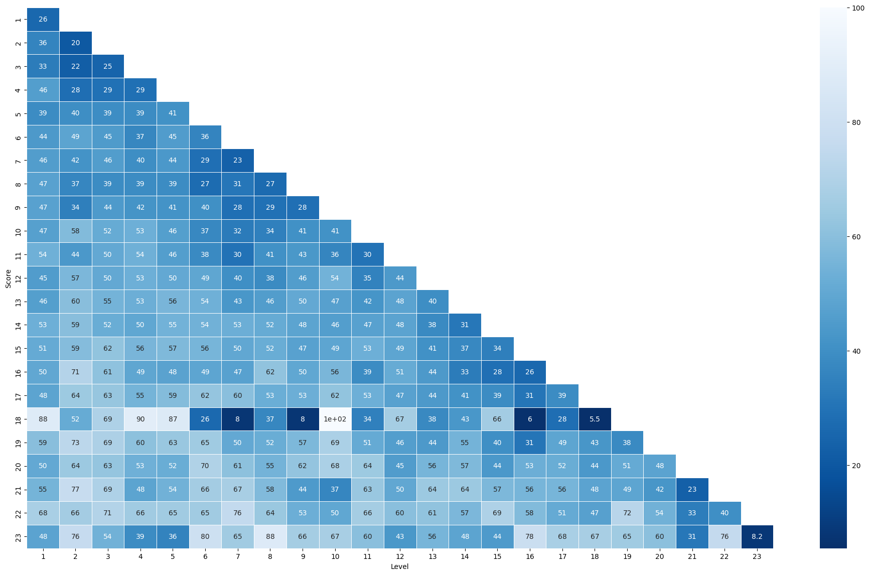
For this race, there is a slightly gradient that gives us an interesting information: for each level it seems that who has gone more on in the race has collected, in average, an higher percentage of \(m\) than the ones who, even if qualified, haven't. It's like there is a direct proportion between collected \(m\) for each level and the progression in the next levels, nevertheless limited to certain ranges.
Another thing that is noteable is a detach in some levels of the group that reached the last level, but we must remember that the average on this row (the number 23) is calculated on a very lower number of records.
The anomalous row (the number 18) is due to the fact that at level 19 there is only one eliminated, therefore is not actually a mean and this messes up a little the information.
You can also do a fill between by noting the "convenience" area of the \(m\) to collect per level, first showing the average of those arriving at the last level.
best_scoring_means| 1 | 2 | 3 | 4 | 5 | 6 | 7 | 8 | 9 | 10 | ... | 14 | 15 | 16 | 17 | 18 | 19 | 20 | 21 | 22 | 23 | |
|---|---|---|---|---|---|---|---|---|---|---|---|---|---|---|---|---|---|---|---|---|---|
| 1 | 26.0 | NaN | NaN | NaN | NaN | NaN | NaN | NaN | NaN | NaN | ... | NaN | NaN | NaN | NaN | NaN | NaN | NaN | NaN | NaN | NaN |
| 2 | 35.8 | 20.461538 | NaN | NaN | NaN | NaN | NaN | NaN | NaN | NaN | ... | NaN | NaN | NaN | NaN | NaN | NaN | NaN | NaN | NaN | NaN |
| 3 | 32.8 | 22.153846 | 24.583333 | NaN | NaN | NaN | NaN | NaN | NaN | NaN | ... | NaN | NaN | NaN | NaN | NaN | NaN | NaN | NaN | NaN | NaN |
| 4 | 45.8 | 28.230769 | 29.416667 | 29.00 | NaN | NaN | NaN | NaN | NaN | NaN | ... | NaN | NaN | NaN | NaN | NaN | NaN | NaN | NaN | NaN | NaN |
| 5 | 38.8 | 39.692308 | 39.250000 | 38.75 | 41.142857 | NaN | NaN | NaN | NaN | NaN | ... | NaN | NaN | NaN | NaN | NaN | NaN | NaN | NaN | NaN | NaN |
| 6 | 44.2 | 48.538462 | 44.916667 | 37.00 | 45.000000 | 36.000000 | NaN | NaN | NaN | NaN | ... | NaN | NaN | NaN | NaN | NaN | NaN | NaN | NaN | NaN | NaN |
| 7 | 45.6 | 41.538462 | 45.500000 | 39.75 | 43.571429 | 28.529412 | 23.40 | NaN | NaN | NaN | ... | NaN | NaN | NaN | NaN | NaN | NaN | NaN | NaN | NaN | NaN |
| 8 | 47.4 | 36.846154 | 39.000000 | 39.00 | 38.714286 | 27.470588 | 31.10 | 26.9 | NaN | NaN | ... | NaN | NaN | NaN | NaN | NaN | NaN | NaN | NaN | NaN | NaN |
| 9 | 47.4 | 34.000000 | 44.416667 | 42.00 | 41.428571 | 40.235294 | 28.40 | 29.3 | 28.4 | NaN | ... | NaN | NaN | NaN | NaN | NaN | NaN | NaN | NaN | NaN | NaN |
| 10 | 46.8 | 58.076923 | 51.500000 | 53.25 | 46.142857 | 37.411765 | 32.50 | 34.4 | 40.8 | 41.142857 | ... | NaN | NaN | NaN | NaN | NaN | NaN | NaN | NaN | NaN | NaN |
| 11 | 53.6 | 43.769231 | 50.166667 | 53.75 | 45.714286 | 38.058824 | 29.65 | 40.8 | 43.2 | 36.428571 | ... | NaN | NaN | NaN | NaN | NaN | NaN | NaN | NaN | NaN | NaN |
| 12 | 45.2 | 56.769231 | 50.250000 | 53.25 | 50.142857 | 49.117647 | 40.15 | 38.4 | 45.6 | 54.428571 | ... | NaN | NaN | NaN | NaN | NaN | NaN | NaN | NaN | NaN | NaN |
| 13 | 46.2 | 59.615385 | 54.750000 | 53.00 | 56.000000 | 53.823529 | 43.00 | 45.5 | 50.4 | 47.142857 | ... | NaN | NaN | NaN | NaN | NaN | NaN | NaN | NaN | NaN | NaN |
| 14 | 53.4 | 59.384615 | 52.166667 | 49.75 | 54.571429 | 53.882353 | 52.80 | 51.6 | 48.4 | 45.857143 | ... | 31.384615 | NaN | NaN | NaN | NaN | NaN | NaN | NaN | NaN | NaN |
| 15 | 51.0 | 58.769231 | 61.833333 | 56.00 | 57.285714 | 55.529412 | 50.10 | 52.0 | 47.4 | 48.714286 | ... | 37.230769 | 34.000000 | NaN | NaN | NaN | NaN | NaN | NaN | NaN | NaN |
| 16 | 50.0 | 71.000000 | 60.916667 | 49.25 | 47.857143 | 48.882353 | 47.20 | 61.5 | 49.6 | 56.142857 | ... | 32.846154 | 28.466667 | 25.8 | NaN | NaN | NaN | NaN | NaN | NaN | NaN |
| 17 | 48.4 | 64.384615 | 62.833333 | 55.00 | 58.571429 | 62.411765 | 60.05 | 52.6 | 52.8 | 61.714286 | ... | 41.076923 | 38.800000 | 30.8 | 38.8 | NaN | NaN | NaN | NaN | NaN | NaN |
| 18 | 88.0 | 51.538462 | 69.166667 | 90.00 | 87.142857 | 26.470588 | 8.00 | 37.0 | 8.0 | 100.000000 | ... | 43.076923 | 66.000000 | 6.0 | 28.0 | 5.454545 | NaN | NaN | NaN | NaN | NaN |
| 19 | 59.4 | 73.230769 | 68.916667 | 60.50 | 63.428571 | 65.058824 | 50.35 | 52.3 | 56.8 | 68.571429 | ... | 54.692308 | 39.866667 | 30.9 | 48.8 | 42.636364 | 38.266667 | NaN | NaN | NaN | NaN |
| 20 | 50.4 | 64.076923 | 62.666667 | 53.50 | 52.285714 | 70.058824 | 60.85 | 54.8 | 62.2 | 68.285714 | ... | 57.230769 | 43.600000 | 53.0 | 52.0 | 43.636364 | 51.200000 | 48.285714 | NaN | NaN | NaN |
| 21 | 55.2 | 76.769231 | 69.083333 | 48.50 | 54.000000 | 66.058824 | 67.45 | 57.7 | 44.4 | 36.571429 | ... | 64.076923 | 57.133333 | 55.5 | 55.6 | 48.272727 | 48.800000 | 42.428571 | 22.916667 | NaN | NaN |
| 22 | 67.6 | 66.153846 | 70.666667 | 65.50 | 65.428571 | 65.352941 | 75.50 | 63.8 | 52.8 | 49.714286 | ... | 56.769231 | 69.066667 | 58.0 | 51.2 | 47.090909 | 72.000000 | 54.000000 | 33.250000 | 39.818182 | NaN |
| 23 | 48.0 | 76.000000 | 54.166667 | 38.75 | 35.714286 | 79.705882 | 65.40 | 87.8 | 66.4 | 67.428571 | ... | 48.307692 | 44.333333 | 78.5 | 67.6 | 67.454545 | 65.066667 | 60.142857 | 31.333333 | 75.636364 | 8.166667 |
23 rows × 23 columns
from plotly.offline import init_notebook_mode, iplot, plot
import plotly.graph_objs as go
import plotly.express as px

y: List[float] = []

for i in range(0, 23):
    y.append(round(best_scoring_means.iloc[22, i], 0))

max_y: List[int] = list(map(lambda i: round(best_scoring_means[i].max()), range(1, 24)))
min_y: List[int] = list(map(lambda i: round(best_scoring_means[i].min()), range(1, 24)))

trace1 = go.Scatter(
                    x = np.linspace(1, 23, 23),
                    y = y,
                    mode = "lines+markers",
                    name = "Mean of collected coins in % by who reached level 23",
                    marker = dict(color = 'rgb(150, 80, 2)'),
                    text= None)

trace2 = go.Scatter(
    x = np.linspace(1, 23, 23),
    y = max_y,
    name = "Max mean of collected coins in %",
    fill='tozeroy', fillcolor='rgba(171, 50, 96, 0.3)',
    marker=dict(color='rgba(171, 50, 96, 0.3)')
)

"""
trace2 = go.Histogram(
    x = min_max_df["max"],
    opacity=0.75,
    xbins=dict(size=1),
    name = "Max mean of collected coins in %",
    marker=dict(color='rgba(171, 50, 96, 0.6)'))
"""

trace3 = go.Scatter(
    x = np.linspace(1, 23, 23),
    y = min_y,
    name = "Min mean of collected coins in %",
    fill='tozeroy', fillcolor='rgba(50, 96, 171, 0.3)',
    marker=dict(color='rgba(50, 96, 171, 0.3)')
)

data = [trace2,trace3,trace1]
layout = dict(barmode='overlay', title = 'Mean of collected coins in %',
              yaxis=dict(title="m %", ticksuffix="%"),
              xaxis= dict(title= 'Level',ticklen=5, nticks=25, tickprefix="L", zeroline= False, range=[0.5,23.5])
             )
fig = dict(data = data, layout = layout)
iplot(fig)
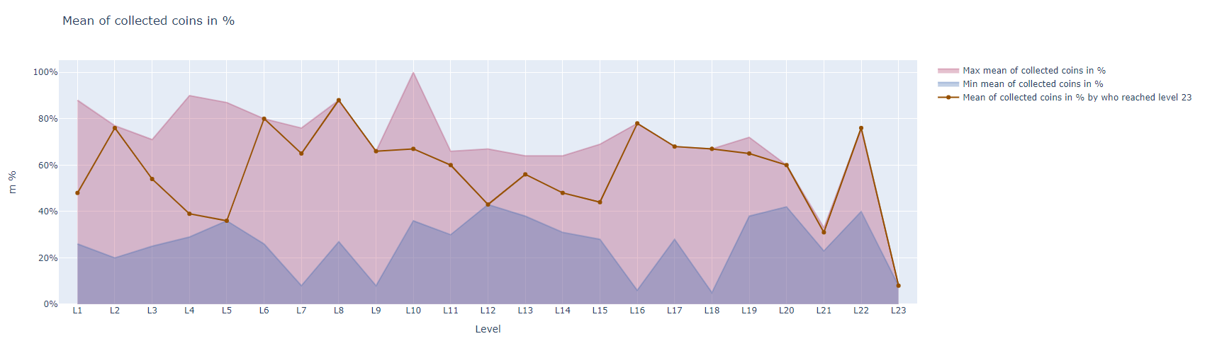
The observations that follow are similar each time the notebook is executed, even if random values are different.
We are able to observe that by average the iterations that reached level 23 are often among those who collected averagly the higher number of coins. But, how much is this "higher number"? The player should consider this because it doesn't mean moving towards 100% of collectable coins at each level, rather it seems to be, often, a percentage between 40% and 80%.
Random Forest training
Final dataset
First thing, the model must be trained on the statistics performed by the best scorers, so the mean of \(m\) collected by those who reached at least level 23, or level 22, or just level 21... I mean the better performing iterations.
Therefore, we will repeat the race many times, each time registering the mean of the best scorers and the score of others. So each race will represent a row in the definitive dataset that will train the model. The mean, or the scores, of the players by reached level will be the parameters, while the score of the best scorers will be the value that has to be predicted.
import pandas as pd

final_dataframe = pd.DataFrame()

def generate_best_scoring_means(race_dataframe: pd.DataFrame, min_score: int) -> pd.DataFrame:
    _best_scoring_means = pd.DataFrame()

    for j in range(1, 24):
        mean: float = round(race_dataframe[race_dataframe["Score"] >= min_score]["m_" + str(j)].mean(), 1)
        _best_scoring_means.loc[0, j] = mean

    return _best_scoring_means

def perform_race() -> pd.DataFrame:
    race_dataframe = pd.DataFrame(data=[])

    """ Initialize participants """
    for i in range(0, competitors):
        race_dataframe.loc[i, 'Iteration'] = i
        race_dataframe.loc[i, 'Score'] = 0
        race_dataframe.loc[i, 'Eliminated'] = False
        race_dataframe['Iteration'] = race_dataframe['Iteration'].astype('int64')
        race_dataframe['Score'] = race_dataframe['Score'].astype('int64')

    for i in range(1, 24):
        race_dataframe = race_level(i, race_dataframe)

    """Take only who reached at least level 21"""
    return generate_best_scoring_means(race_dataframe, 21)

for i in range(0, 100):
    print("Executing iteration", i)
    i_df = perform_race()
    final_dataframe = pd.concat([final_dataframe, i_df])
    final_dataframe = final_dataframe.reset_index(drop=True)

final_dataframe
Executing iteration 0
Executing iteration 1
Executing iteration 2
Executing iteration 3
Executing iteration 4
Executing iteration 5
Executing iteration 6
Executing iteration 7
Executing iteration 8
Executing iteration 9
Executing iteration 10
Executing iteration 11
Executing iteration 12
Executing iteration 13
Executing iteration 14
Executing iteration 15
Executing iteration 16
Executing iteration 17
Executing iteration 18
Executing iteration 19
Executing iteration 20
Executing iteration 21
Executing iteration 22
Executing iteration 23
Executing iteration 24
Executing iteration 25
Executing iteration 26
Executing iteration 27
Executing iteration 28
Executing iteration 29
Executing iteration 30
Executing iteration 31
Executing iteration 32
Executing iteration 33
Executing iteration 34
Executing iteration 35
Executing iteration 36
Executing iteration 37
Executing iteration 38
Executing iteration 39
Executing iteration 40
Executing iteration 41
Executing iteration 42
Executing iteration 43
Executing iteration 44
Executing iteration 45
Executing iteration 46
Executing iteration 47
Executing iteration 48
Executing iteration 49
Executing iteration 50
Executing iteration 51
Executing iteration 52
Executing iteration 53
Executing iteration 54
Executing iteration 55
Executing iteration 56
Executing iteration 57
Executing iteration 58
Executing iteration 59
Executing iteration 60
Executing iteration 61
Executing iteration 62
Executing iteration 63
Executing iteration 64
Executing iteration 65
Executing iteration 66
Executing iteration 67
Executing iteration 68
Executing iteration 69
Executing iteration 70
Executing iteration 71
Executing iteration 72
Executing iteration 73
Executing iteration 74
Executing iteration 75
Executing iteration 76
Executing iteration 77
Executing iteration 78
Executing iteration 79
Executing iteration 80
Executing iteration 81
Executing iteration 82
Executing iteration 83
Executing iteration 84
Executing iteration 85
Executing iteration 86
Executing iteration 87
Executing iteration 88
Executing iteration 89
Executing iteration 90
Executing iteration 91
Executing iteration 92
Executing iteration 93
Executing iteration 94
Executing iteration 95
Executing iteration 96
Executing iteration 97
Executing iteration 98
Executing iteration 99| 1 | 2 | 3 | 4 | 5 | 6 | 7 | 8 | 9 | 10 | ... | 14 | 15 | 16 | 17 | 18 | 19 | 20 | 21 | 22 | 23 | |
|---|---|---|---|---|---|---|---|---|---|---|---|---|---|---|---|---|---|---|---|---|---|
| 0 | 27.2 | 90.3 | 82.1 | 22.3 | 40.1 | 121.0 | 133.2 | 62.7 | 24.3 | 42.9 | ... | 84.5 | 83.4 | 58.7 | 24.6 | 60.8 | 45.7 | 65.9 | 84.5 | 61.9 | 123.8 |
| 1 | 25.8 | 89.8 | 77.7 | 22.5 | 34.1 | 115.2 | 146.6 | 63.7 | 28.8 | 44.3 | ... | 75.0 | 92.2 | 54.8 | 27.2 | 54.7 | 40.6 | 70.7 | 89.0 | 57.2 | 125.1 |
| 2 | 27.6 | 97.3 | 82.4 | 20.4 | 39.2 | 101.1 | 142.2 | 60.8 | 30.4 | 42.5 | ... | 78.5 | 88.3 | 45.1 | 23.5 | 62.5 | 39.0 | 69.2 | 65.7 | 60.5 | 177.6 |
| 3 | 29.8 | 89.6 | 80.7 | 23.1 | 41.1 | 110.5 | 150.6 | 57.4 | 28.0 | 38.9 | ... | 81.6 | 84.9 | 54.7 | 19.0 | 58.0 | 36.4 | 62.5 | 72.6 | 57.4 | 153.7 |
| 4 | 27.8 | 91.3 | 72.0 | 23.6 | 38.6 | 122.4 | 140.2 | 61.0 | 23.8 | 38.9 | ... | 72.6 | 74.7 | 39.3 | 24.0 | 53.0 | 36.0 | 63.8 | 69.9 | 66.9 | 165.7 |
| ... | ... | ... | ... | ... | ... | ... | ... | ... | ... | ... | ... | ... | ... | ... | ... | ... | ... | ... | ... | ... | ... |
| 95 | 26.5 | 90.8 | 79.3 | 20.3 | 40.5 | 117.5 | 134.3 | 60.6 | 27.4 | 34.0 | ... | 78.7 | 85.1 | 52.7 | 24.6 | 60.3 | 40.7 | 76.5 | 86.9 | 52.7 | 160.0 |
| 96 | 33.5 | 89.3 | 85.4 | 24.6 | 40.9 | 112.1 | 140.4 | 59.6 | 28.4 | 44.0 | ... | 77.0 | 87.7 | 47.6 | 25.4 | 55.4 | 38.8 | 73.1 | 75.3 | 60.2 | 158.4 |
| 97 | 31.2 | 94.5 | 77.8 | 21.9 | 37.7 | 120.4 | 133.1 | 55.7 | 29.8 | 45.5 | ... | 79.1 | 78.7 | 51.5 | 24.8 | 56.1 | 40.5 | 68.4 | 79.1 | 56.7 | 165.3 |
| 98 | 28.8 | 89.2 | 84.1 | 21.1 | 43.1 | 116.4 | 143.2 | 48.6 | 25.6 | 40.9 | ... | 75.9 | 82.6 | 49.2 | 28.1 | 49.8 | 42.3 | 69.8 | 80.5 | 48.3 | 166.5 |
| 99 | 28.1 | 98.9 | 81.3 | 22.0 | 42.1 | 113.2 | 133.4 | 58.6 | 23.5 | 38.2 | ... | 81.0 | 72.1 | 48.1 | 27.8 | 52.2 | 36.4 | 62.1 | 95.5 | 51.8 | 155.2 |
100 rows × 23 columns
At last... the training
In first instance let's predict the \(m\)s that is convenient to collect at the first level. Than we will repeat this for each level.
To do this we have to understand how to handle all the NaN values, generated by the fact that eliminated players don't collect \(m\) anymore.
from sklearn.model_selection import train_test_split
from sklearn.metrics import log_loss
from sklearn.metrics import accuracy_score
from sklearn.ensemble import RandomForestClassifier

X = race_dataframe.drop("Score", axis=1).values
Y = race_dataframe["Score"].values

X_train, X_test, Y_train, Y_test = train_test_split(X, Y, test_size=0.3, random_state=0)

forest = RandomForestClassifier(n_estimators=30, max_depth=8, random_state=False)

forest.fit(X_train, Y_train)

y_pred_train = forest.predict(X_train)
y_pred = forest.predict(X_test)

accuracy_train = accuracy_score(Y_train, y_pred_train)
accuracy_test = accuracy_score(Y_test, y_pred)

print("ACCURACY: TRAIN=%.4f TEST=%.4f" % (accuracy_train,accuracy_test))
Test the model compete in a race against other 999 randomic players
This work is not yet completed.